Deep learning - from getting started to giving up (VI) introduction to CNN and RNN
1. Introduction of CNN and RNN
- CNN
1. It is mainly used in image processing. CNN is a feedforward neural network through convolution calculation. It is proposed by the receptive field mechanism in biology. It has translation invariance. It uses convolution kernel to maximize the application of local information and retain the plane structure information.
2. Computing resources can be reduced by sharing parameters in space - RNN
1. It is mainly applied to sequence problems related to timing, such as natural language processing (the sentence length in natural language is usually not fixed). We will talk about RNN in a later tutorial. - DNN
DNN here can be understood as the simple neural network we learned before. It is composed of input layer, hidden layer and output layer. Each neuron belongs to different layers. Each neuron is connected with all neurons in the previous layer, and the signal propagates unidirectionally from the input layer to the output layer.
2.CNN
Convolutional neural network (CNN) is a kind of neural network specially used to process data with grid structure. Convolution network refers to those neural networks that use convolution operation to replace the general matrix multiplication operation in at least one layer of the network.
2.1 convolution and edge detection
2.1.1 convolution
In essence, convolution simply multiplies one matrix (called kernel or filter) repeatedly with some other larger matrices (in our example, the pixels of the image).
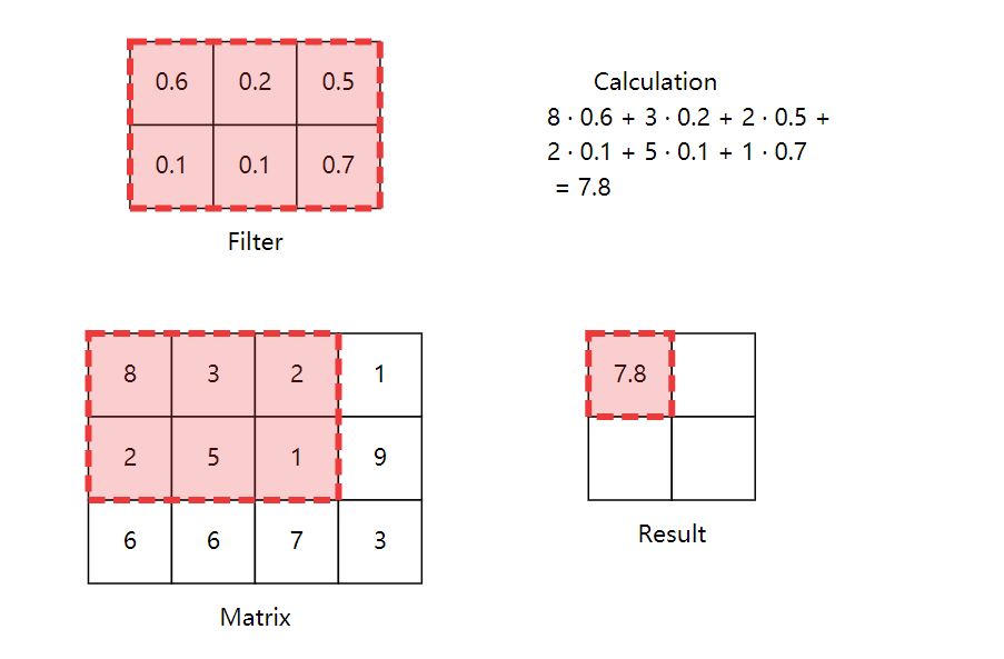
The above figure is an example of a convolution process. Different convolution results can be obtained by changing the size of the filter and the sliding step size.
- In order to better understand the meaning of convolution, we introduce the concept of weight sharing here. The simple understanding of weight sharing is that in the sliding process of the existing filter, the weights in the network are the same, that is, all neurons in the first hidden layer detect the same feature from the input layer, only from different positions of the input layer (middle of picture, upper left corner, lower right corner, etc.)
It is not difficult to see that in CNN, a filter can only extract one spatial feature, so what is the significance of doing so?
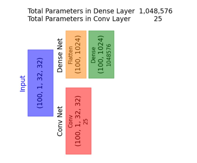
- Weight sharing can greatly reduce the number of model parameters, so as to reduce the computational burden
2.1.2 convolution output size
How will the output shape change after convolution? When you know the shape of the input matrix and convolution kernel, what is the output shape?
- transport Out = transport enter − volume product nucleus + 1 Output = input convolution kernel + 1 Output = input − convolution kernel + 1
2.1.3 demonstrate convolution in PyTorch
Look at the following code. In it, we define a Net class that you can instantiate using the kernel to create a neural network object. When you apply a network object to an image (or anything in the form of a matrix), it convolutes the kernel on the image.
class Net(nn.Module):
  """
 Here we define a CNN Class of
 If we select the corresponding convolution kernel, we can call this class to convolute the image
  i.e. Net(kernel)(image)
  """
  def __init__(self, kernel=None, padding=0):
    super(Net, self).__init__()
    # Summary of the nn.conv2d parameters (you can also get this by hovering
    # over the method):
    # in_channels (int): Number of channels in the input image
    # out_channels (int): Number of channels produced by the convolution
    # kernel_size (int or tuple): Size of the convolving kernel
    # padding (int or tuple, optional): padding is mainly used in the scene of edge detection
    self.conv1 = nn.Conv2d(in_channels=1, out_channels=1, kernel_size=2, \
                           padding=padding)

    # set up a default kernel if a default one isn't provided
    if kernel is not None:
      dim1, dim2 = kernel.shape[0], kernel.shape[1]
      kernel = kernel.reshape(1, 1, dim1, dim2)

      self.conv1.weight = torch.nn.Parameter(kernel)
      self.conv1.bias = torch.nn.Parameter(torch.zeros_like(self.conv1.bias))

  def forward(self, x):
    x = self.conv1(x)
    return x

# Format a default 2x2 kernel of numbers from 0 through 3
kernel = torch.Tensor(np.arange(4).reshape(2, 2))
# Prepare the network with that default kernel
net = Net(kernel=kernel, padding=0).to(DEVICE)

# set up a 3x3 image matrix of numbers from 0 through 8
image = torch.Tensor(np.arange(9).reshape(3, 3))
image = image.reshape(1, 1, 3, 3).to(DEVICE) # BatchSizeXChannelsXHeightXWidth

print("Image:\n" + str(image))
print("Kernel:\n" + str(kernel))
output = net(image) # Apply the convolution
print("Output:\n" + str(output))
Image:
tensor([[[[0., 1., 2.],
[3., 4., 5.],
[6., 7., 8.]]]])
Kernel:
tensor([[0., 1.],
[2., 3.]])
Output:
tensor([[[[19., 25.],
[37., 43.]]]], grad_fn=)
We can find that the input size is 3 × 3. The output size is 2 × 2. This is because the kernel cannot generate values for the edges of the image - when it slides to the end of the image and centered on the boundary pixels, it will overlap the undefined space outside the image. If we don't want to lose this information, we will have to fill the image with some default values (such as 0) on the border. Predictably, this process is called padding.
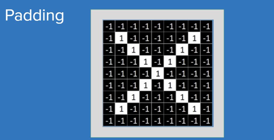
The gray part in the figure above is the pixel filled with the default value. Based on this feature of padding, it is also used for edge detection.
- padding adds the default value to the outer edge of the image
- The step size adjusts the distance the filter moves after each convolution.
2.2 pooling and down sampling
Before talking about pooling, let's review the filter in convolution. The information of the image after convolution will not change and still maintain global invariance. Imagine a scenario: if we want to use CNN to identify vehicles, in the face of different tire sizes of different vehicles, we certainly don't want our network just because of wheels At this time, the application of pooling can reduce the local recognition sensitivity, that is, pooling can bring local invariance.
2.2.1 case introduction
1. Data preparation
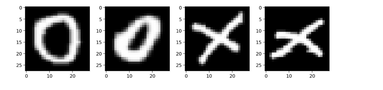
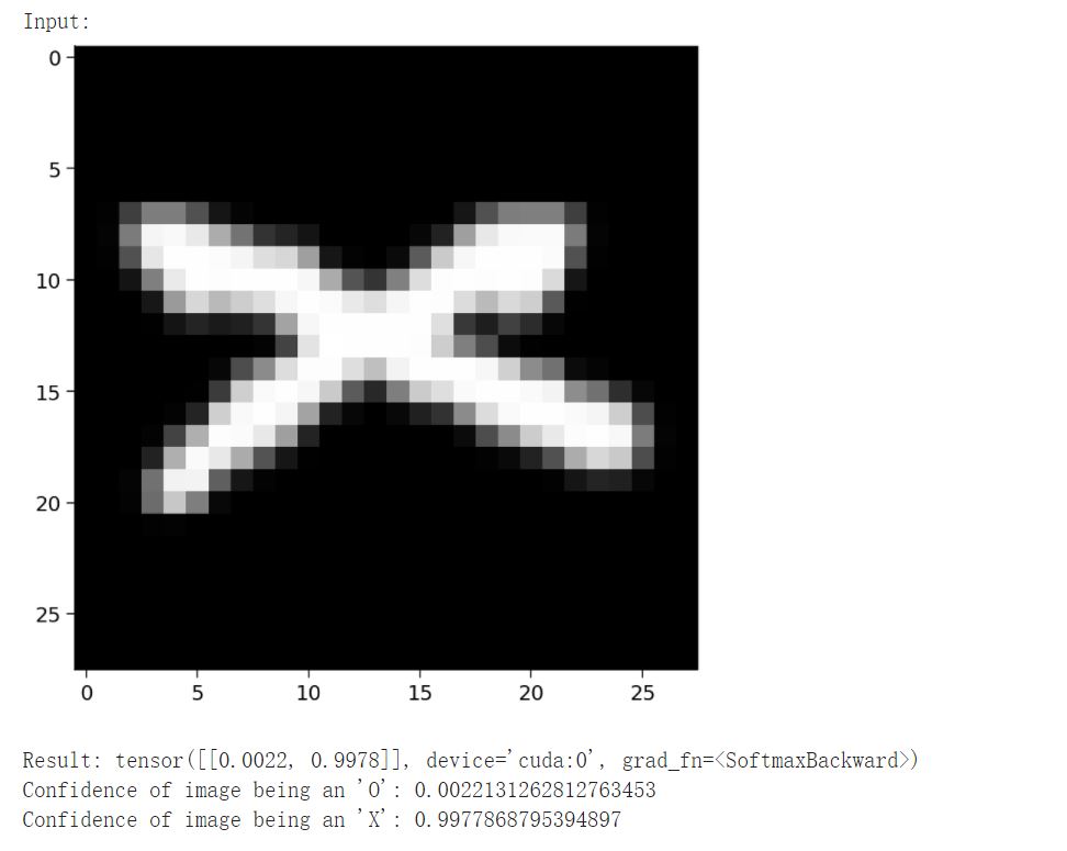
In order to visualize the various components of CNN, we will gradually build A simple CNN. We will use EMNIST alphabet dataset, which consists of binary images of handwritten characters (A,..., Z). We will train A CNN to classify the images X or O.
2. Multiple convolution kernels are used for convolution at the same time
class Net2(nn.Module):
  def __init__(self, padding=0):
    super(Net2, self).__init__()
    self.conv1 = nn.Conv2d(in_channels=1, out_channels=3, kernel_size=5,
                           padding=padding)

    # First convolution kernel - principal diagonal
    kernel_1 = torch.Tensor([[[ 1.,  1., -1., -1., -1.],
                              [ 1.,  1.,  1., -1., -1.],
                              [-1.,  1.,  1.,  1., -1.],
                              [-1., -1.,  1.,  1.,  1.],
                              [-1., -1., -1.,  1.,  1.]]])

    # Second convolution kernel - other diagonal
    kernel_2 = torch.Tensor([[[-1., -1., -1.,  1.,  1.],
                              [-1., -1.,  1.,  1.,  1.],
                              [-1.,  1.,  1.,  1., -1.],
                              [ 1.,  1.,  1., -1., -1.],
                              [ 1.,  1., -1., -1., -1.]]])

    # Third convolution kernel checkerboard pattern
    kernel_3 = torch.Tensor([[[ 1.,  1., -1.,  1.,  1.],
                              [ 1.,  1.,  1.,  1.,  1.],
                              [-1.,  1.,  1.,  1., -1.],
                              [ 1.,  1.,  1.,  1.,  1.],
                              [ 1.,  1., -1.,  1.,  1.]]])


    # Stack all kernels in one tensor with (3, 1, 5, 5) dimensions
    multiple_kernels = torch.stack([kernel_1, kernel_2, kernel_3], dim=0)

    self.conv1.weight = torch.nn.Parameter(multiple_kernels)
    # Negative bias
    self.conv1.bias = torch.nn.Parameter(torch.Tensor([-4, -4, -12]))

  def forward(self, x):
    x = self.conv1(x)
    return x
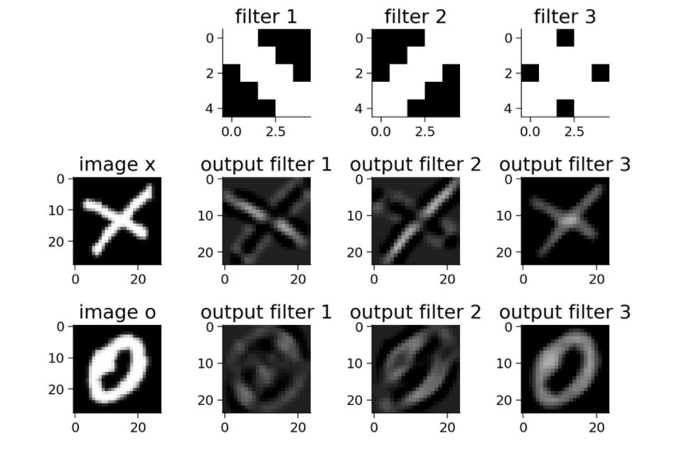
It is not difficult to see from the above figure that these filters are customized to respond strongly to X; diagonal edge filters emphasize
The two diagonals that make up x are the center of the checkerboard pattern to X.
3. RLU after convolution
So far, we have discussed convolution operation, which is linear. But the real advantage of neural network comes from the combination of nonlinear functions. In addition, in the real world, we often encounter nonlinear and complex learning problems between input and output.
ReLU (modified linear unit) introduces nonlinearity into our model, so that we can learn more complex functions and better predict the category of images. ReLU is mentioned in the previous tutorial and will not be repeated here.
class Net3(nn.Module):
  def __init__(self, padding=0):
    super(Net3, self).__init__()
    self.conv1 = nn.Conv2d(in_channels=1, out_channels=3, kernel_size=5,
                           padding=padding)

    # First convolution kernel - principal diagonal
    kernel_1 = torch.Tensor([[[ 1.,  1., -1., -1., -1.],
                              [ 1.,  1.,  1., -1., -1.],
                              [-1.,  1.,  1.,  1., -1.],
                              [-1., -1.,  1.,  1.,  1.],
                              [-1., -1., -1.,  1.,  1.]]])

    # Second convolution kernel - other diagonal
    kernel_2 = torch.Tensor([[[-1., -1., -1.,  1.,  1.],
                              [-1., -1.,  1.,  1.,  1.],
                              [-1.,  1.,  1.,  1., -1.],
                              [ 1.,  1.,  1., -1., -1.],
                              [ 1.,  1., -1., -1., -1.]]])

    # Third convolution kernel checkerboard pattern
    kernel_3 = torch.Tensor([[[ 1.,  1., -1.,  1.,  1.],
                              [ 1.,  1.,  1.,  1.,  1.],
                              [-1.,  1.,  1.,  1., -1.],
                              [ 1.,  1.,  1.,  1.,  1.],
                              [ 1.,  1., -1.,  1.,  1.]]])


    # Stack all kernels in one tensor with (3, 1, 5, 5) dimensions
    multiple_kernels = torch.stack([kernel_1, kernel_2, kernel_3], dim=0)

    self.conv1.weight = torch.nn.Parameter(multiple_kernels)
    # Negative bias
    self.conv1.bias = torch.nn.Parameter(torch.Tensor([-4, -4, -12]))

  def forward(self, x):
    x = self.conv1(x)
    x = F.relu(x)#Introducing ReLU
    return x
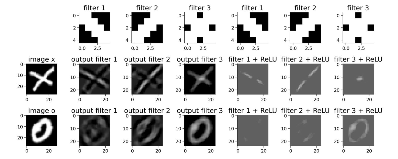
After the introduction of ReLU, the response of our filter to X becomes more obvious, and the extracted three spatial features are also perfectly displayed. Therefore, using ReLU can better identify the image.
2.2.2 pooling
The convolution layer creates feature maps to summarize the existence of specific features (such as edges) in the input. However, these feature maps record the exact position of features in the input. This means that small changes in the position of objects in the image may lead to very different feature maps. Therefore, we need to achieve translation invariance.
A common method to solve this problem is called downsampling. Downsampling creates a lower resolution version of the image, preserves large structural elements and deletes some fine details that may not be relevant to the task. In CNN, maximum pooling and average pooling are used for downsampling. These operations reduce the size of hidden layers and produce more translation invariant features, and subsequent layers can be better Make good use of these features.
Like the convolution layer, the pooling layer has fixed shaped windows (pooling windows), which are systematically applied to the input. Like filters, we can change the shape of the window and the size of the stride. And, like filters, every time we apply a pooling operation, we produce an output.
Pooling performs an information compression that provides summary statistics for the input neighborhood. After pooling, the eigenvalues we learned are greatly reduced, and the parameters of the later network layer are greatly reduced
- In Maxpooling, we calculate the maximum value of all pixels in the pooled window.
- In Avgpooling, we calculate the average of all pixels in the pooled window.
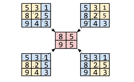
The figure above shows an example of Max pooling.
2.2.3 implementing MaxPooling
Now let's implement MaxPooling in PyTorch and observe the impact of Pooling on the dimension of the input image. Use a kernel with a size of 2 and a step size of 2 for the MaxPooling layer.
class Net4(nn.Module):
  def __init__(self, padding=0, stride=2):
    super(Net4, self).__init__()
    self.conv1 = nn.Conv2d(in_channels=1, out_channels=3, kernel_size=5,
                            padding=padding)

    # first kernel - leading diagonal
    kernel_1 = torch.Tensor([[[ 1.,  1., -1., -1., -1.],
                              [ 1.,  1.,  1., -1., -1.],
                              [-1.,  1.,  1.,  1., -1.],
                              [-1., -1.,  1.,  1.,  1.],
                              [-1., -1., -1.,  1.,  1.]]])

    # second kernel - other diagonal
    kernel_2 = torch.Tensor([[[-1., -1., -1.,  1.,  1.],
                              [-1., -1.,  1.,  1.,  1.],
                              [-1.,  1.,  1.,  1., -1.],
                              [ 1.,  1.,  1., -1., -1.],
                              [ 1.,  1., -1., -1., -1.]]])

    # third kernel -checkerboard pattern
    kernel_3 = torch.Tensor([[[ 1.,  1., -1.,  1.,  1.],
                              [ 1.,  1.,  1.,  1.,  1.],
                              [-1.,  1.,  1.,  1., -1.],
                              [ 1.,  1.,  1.,  1.,  1.],
                              [ 1.,  1., -1.,  1.,  1.]]])


    # Stack all kernels in one tensor with (3, 1, 5, 5) dimensions
    multiple_kernels = torch.stack([kernel_1, kernel_2, kernel_3], dim=0)

    self.conv1.weight = torch.nn.Parameter(multiple_kernels)
    # Negative bias
    self.conv1.bias = torch.nn.Parameter(torch.Tensor([-4, -4, -12]))
    self.pool = nn.MaxPool2d(kernel_size=2, stride=stride)#Apply Max pooling

  def forward(self, x):
    x = self.conv1(x)
    x = F.relu(x)
    x = self.pool(x)  # pass through a max pool layer
    return x
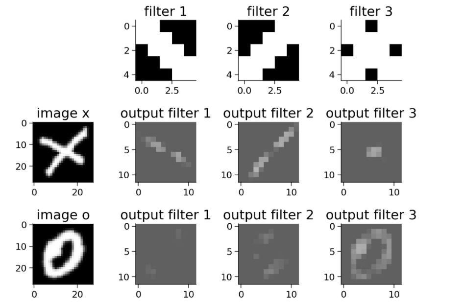
We can observe that the size of the output is half the size seen after the ReLU part, which is caused by the Maxpool layer. Although the size of the output is reduced, the important or advanced features in the output remain unchanged.
3. Build a CNN network
3.1CNN consists of five structures
- Input layer: the input layer generally represents the pixel matrix of a picture. You can use a three-dimensional matrix to represent a picture. The length and width of the three-dimensional matrix represent the size of the image, while the depth of the three-dimensional matrix represents the color channel of the image. [Channels, Height, Width]
- Convolution layer
- Pooling layer
- Full connection layer: after multiple rounds of convolution layer and pool layer processing, the final classification results are generally given by 1 to 2 full connection layers at the end of CNN.
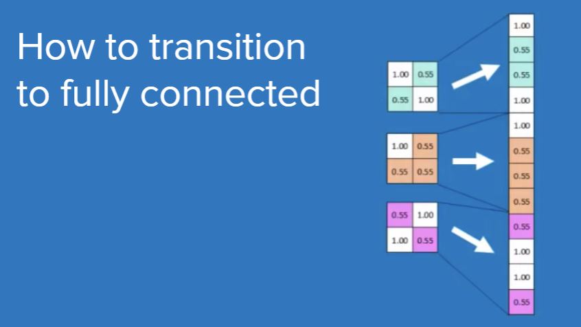
Note: the operation of flatten is required from the pool layer to the full connection layer - Softmax layer: through the softmax layer, you can get the probability distributions of the current sample belonging to different types.
3.2 network architecture
Convolution nn.Conv2d(in_channels=1, out_channels=32, kernel_size=3)
Convolution nn.Conv2d(in_channels=32, out_channels=64, kernel_size=3)
Pooling layer nn.MaxPool2d(kernel_size=2)
Full connection layer nn.Linear(in_features=9216, out_features=128)
Full connection layer nn.Linear(in_features=128, out_features=2)
class EMNIST_Net(nn.Module):
  def __init__(self):
    super(EMNIST_Net, self).__init__()
    #The size of the input image is [28, 28]
    #The input image Chanel=1, the number of filter s generated after convolution is 32, and the convolution kernel is 3 * 3
    self.conv1 = nn.Conv2d(1, 32, 3)
    #The input image Chanel=32, the number of filter s generated after convolution is 64, and the convolution kernel is 3 * 3
    self.conv2 = nn.Conv2d(32, 64, 3)
    #The image size after twice convolution becomes 28-3 + 1-3 + 1 = 24 - > [24,24]. After Max pooling and introducing ReLU, the output size becomes half of the original, that is [12,12]. At this time, the image size is 12 * 12 = 128
    #We want to flatten the output of the convolution layer before transferring the linear layer, so as to convert the input of the shape [BatchSize, Channels, Height, Width] into [BatchSize, Channels\*Height\ *Width]. In this case, from [32, 64, 12, 12] (the output of the second convolution layer) to [32, 64 * 12 * 12] = [32, 9216].
    self.fc1 = nn.Linear(9216, 128)
    self.fc2 = nn.Linear(128, 2)#The number of final categories is 2
    self.pool = nn.MaxPool2d(2)

  def forward(self, x):
    x = self.conv1(x)
    x = F.relu(x)
    x = self.conv2(x)
    x = F.relu(x)
    x = self.pool(x)
    x = torch.flatten(x, 1)
    x = self.fc1(x)
    x = F.relu(x)
    x = self.fc2(x)
    return x


# add event to airtable
atform.add_event('Coding Exercise 4: Implement your own CNN')

## Uncomment the lines below to train your network
emnist_net = EMNIST_Net().to(DEVICE)
print("Total Parameters in Network {:10d}".format(sum(p.numel() for p in emnist_net.parameters())))
train(emnist_net, DEVICE, train_loader, 1)
Welcome to the public official account.