Deep learning image classification (11) mobile netv2 network structure

In this section, learn about the network structure of MobileNetV2. Learning video from Bilibili , part of the reference description is derived from knowhow Explain MobileNetV2 in detail.

1. Preface

MobileNetV2 was proposed by the google team in 2018. Compared with MobileNetV1, it has higher accuracy and smaller model. Its original paper is MobileNetV2: Inverted Residuals and Linear Bottlenecks.

We found that many DW convolution weights in MobileNetV1 are 0, which is actually invalid. A very important reason is that the gradient of the ReLU activation function to the value of 0 is 0, and the value of this node will not be recovered no matter how it is iterated later. Therefore, if the value of the node becomes 0, it will "die". The residual structure of ResNet can alleviate this feature degradation problem to a great extent. Therefore, it is natural for MobileNetV2 to try to introduce the Residuals module and study the ReLU activation function. The motivation is quite clear and the story is very clear.

Highlights in MobileNetV2 network (just the name of the paper) include:

• Inverted Residuals structure
• Linear Bottlenecks

2. Inverted Residuals structure

First, let's take a look at the Inverted Residuals structure. In the Residuals structure proposed by ResNet, first use 1 × 1 1 \times 1 one × 1 convolution to reduce the dimension, and then 3 × 3 3 \times 3 three × 3 convolution, finally through 1 × 1 1 \times 1 one × 1 convolution realizes dimension upgrading, that is, the two ends are large and the middle is small. In MobileNetV2, the order of dimensionality reduction and upgrading is changed, and 3 × 3 3 \times 3 three × 3 convolution is replaced by 3 × 3 3 \times 3 three × 3 DW convolution, that is, the two ends are small and the middle is large.

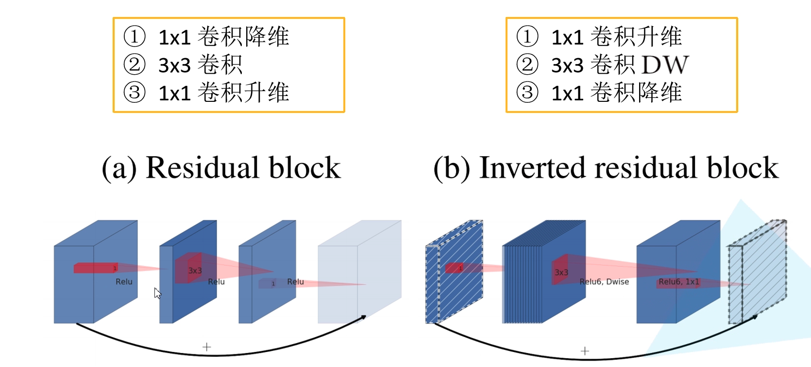
In addition, the activation function is also different. In Inverted Residuals, the ReLU6 activation function is used, and its expression is y = ReLU ( 6 ) = m i n ( m a x ( x , 0 ) , 6 ) y = \text{ReLU}(6) = min(max(x,0), 6) y=ReLU(6)=min(max(x,0),6).

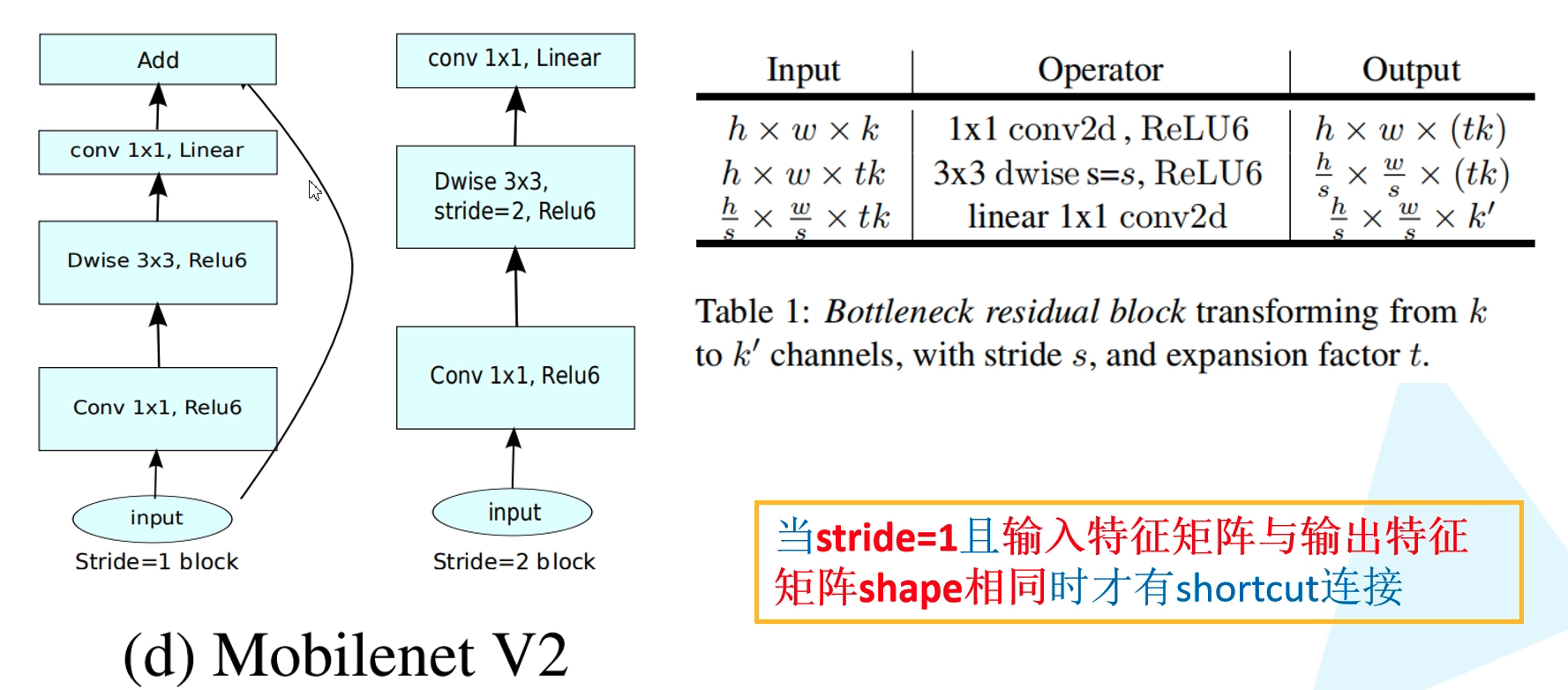
The structure diagram of Inverted Residuals in MobileNetV2 is as follows. Unlike ResNet, there is a shortcut connection only when stripe = 1 and the input characteristic matrix is the same as the output characteristic matrix shape.

The core problem of the Inverted Residuals structure is: why do you want to increase the dimension and then reduce the dimension?

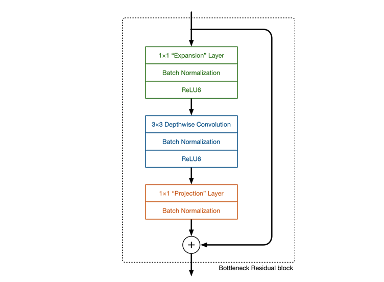
The main idea of MobileNetV1 network is the stacking of deep separable convolution, which is basically consistent with the stacking idea of VGG. In addition to DW convolution structure, the Inverted Residuals structure also uses Expansion layer and Projection layer. This Projection layer uses 1 × 1 1 \times 1 one × The purpose of convolution network structure is to map high-dimensional features to low-dimensional space. To add, use 1 × 1 1 \times 1 one × The design of convolution network structure mapping high-dimensional space to low-dimensional space is sometimes called Bottleneck layer. The function of Expansion layer is just the opposite 1 × 1 1 \times 1 one × 1 convolution network structure, which aims to map low-dimensional space to high-dimensional space. Here, the Expansion has a super parameter, which is several times the dimension Expansion. It can be adjusted according to the actual situation. The default value is 6, that is, it is expanded by 6 times.

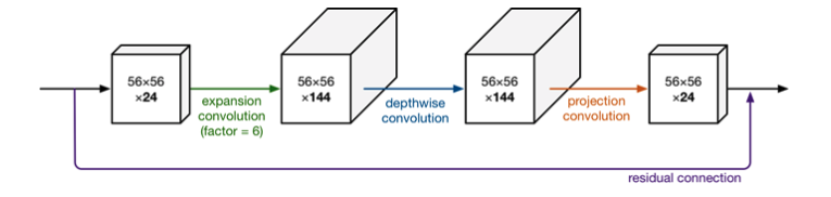
We know that the lower the Tensor dimension, the smaller the amount of multiplication / addition calculation in the convolution layer. If the whole network is low dimensional Tensor, the overall computing speed will be very fast (this is consistent with the original intention of MobileNet). However, If you only use low dimensional Tensor, the effect will not be good (the article MEPDNet in ICIP2021 mentioned the inverted triangle, which is not to increase the dimension, but to increase the size). If the filter s of the convolution layer use low-dimensional Tensor to extract features, there is no way to extract enough information of the whole. Therefore, if we extract feature data, we may prefer high-dimensional Tensor to do this. Total In conclusion, when there is no way to determine whether these features are sufficient or complete, you should choose more features to use. The more Han Xin recruits, the better. MobileNetV2 designed such a structure to achieve balance.

First, expand the dimension through the Expansion layer, then extract the features with the depth separable convolution, and then use the Projection layer to compress the data to make the network smaller. Because both Expansion layer and Projection layer have parameters that can be learned, the whole network structure can learn how to better expand and compress data. Why didn't the original structure rise first and then fall? Simple, because among them 3 × 3 3 \times 3 three × 3 too much convolution calculation. The reason why MobileNetV2 dares to do this is that DW convolution has a small amount of calculation. If the middle is ordinary convolution and the amount of calculation is too large, it is necessary to reduce the dimension first and then increase the dimension to reduce the amount of calculation and parameters.

3. Linear Bottlenecks

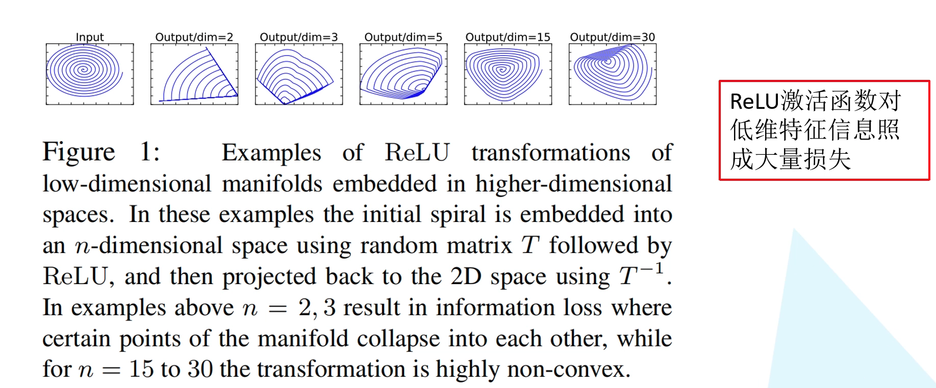
In the original text, the author aims at the last part of the Inverted Residuals structure 1 × 1 1 \times 1 one × 1 the convolution uses the linear activation function instead of the ReLU activation function. The author did an experiment to illustrate this. First, the input is a two-dimensional matrix, channel = 1. We use different matrices T T T upgrades it to a higher dimension, uses the activation function ReLU, and then uses T T Inverse matrix of T T − 1 T^{-1} Restore it with T − 1. When T T When the dimension of T is 2 or 3, a lot of information is lost after restoring to the 2D characteristic matrix. However, with the increase of dimensions, less and less information is lost. It can be seen that the ReLU activation function will cause a large loss of low dimensional feature information. Because the two ends of the Inverted Residuals structure are small and the middle is large, it is a low dimensional feature at the last output, so it is changed to a linear activation function instead of a ReLU activation function. Experiments show that using linear bottleneck can prevent nonlinear destruction of too much information.

4. MobileNetV2 network structure

The following figure shows the network structure configuration diagram of MobileNetV2. Where t is in the Inverted Residuals structure 1 × 1 1 \times 1 one × 1 the magnification of the convolution dimension (compared with the input channel), c is the depth channel of the output characteristic matrix. n indicates the number of repetitions of bottleneck (i.e. Inverted Residuals structure). s represents the step length, but it only represents the step length of DW convolution in the first bottleneck, and the stripe of repeated bottleneck is equal to 1.

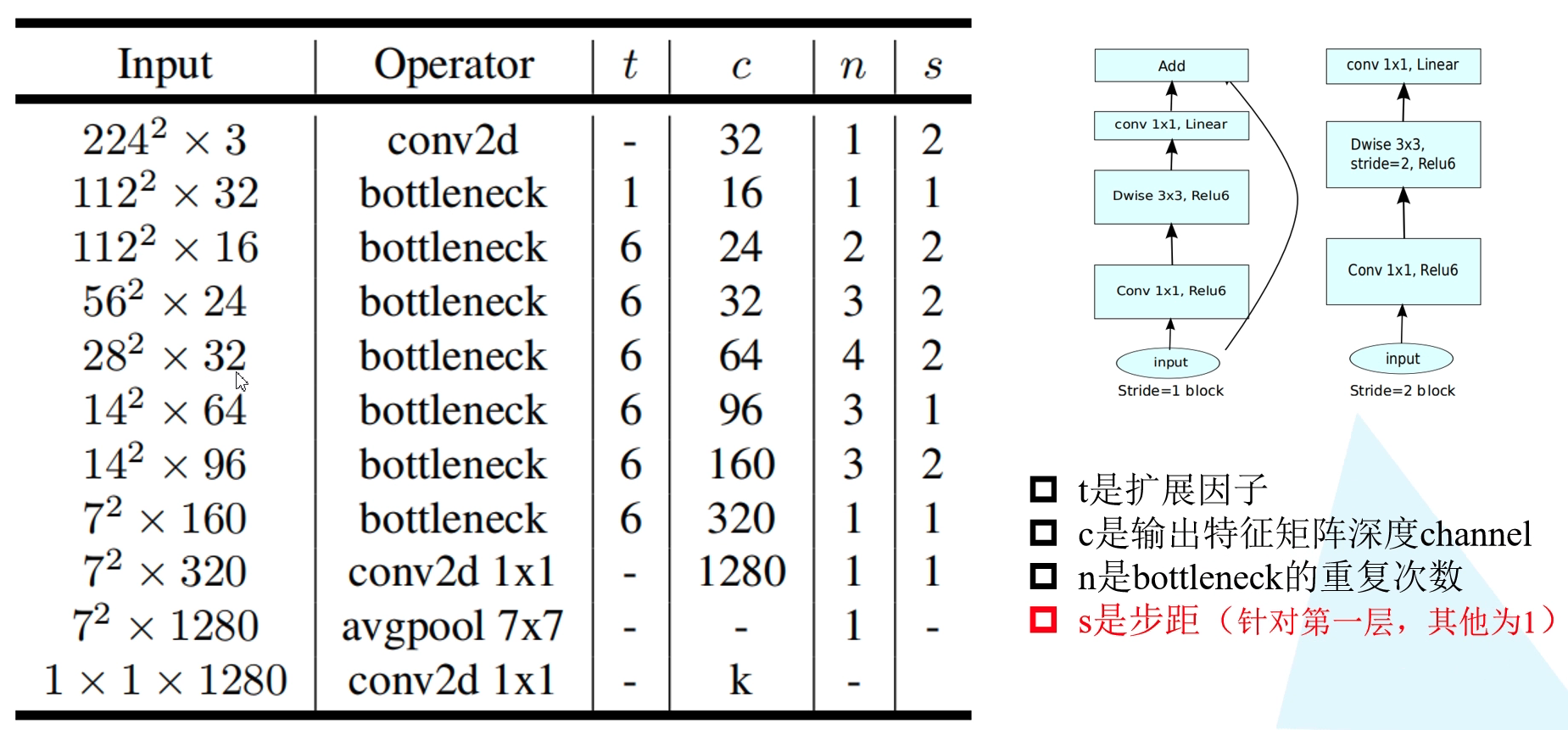
It is worth noting that in the official implementation of pytorch and tensorflow, the first bottleneck is useless 1 × 1 1 \times 1 one × 1 convolution, but directly connected to DW convolution. Because the expansion factor of this in the original paper t = 1 t = 1 t=1, that is, even if it is used 1 × 1 1 \times 1 one × 1 convolution does not increase the dimension. So it's no use at all.

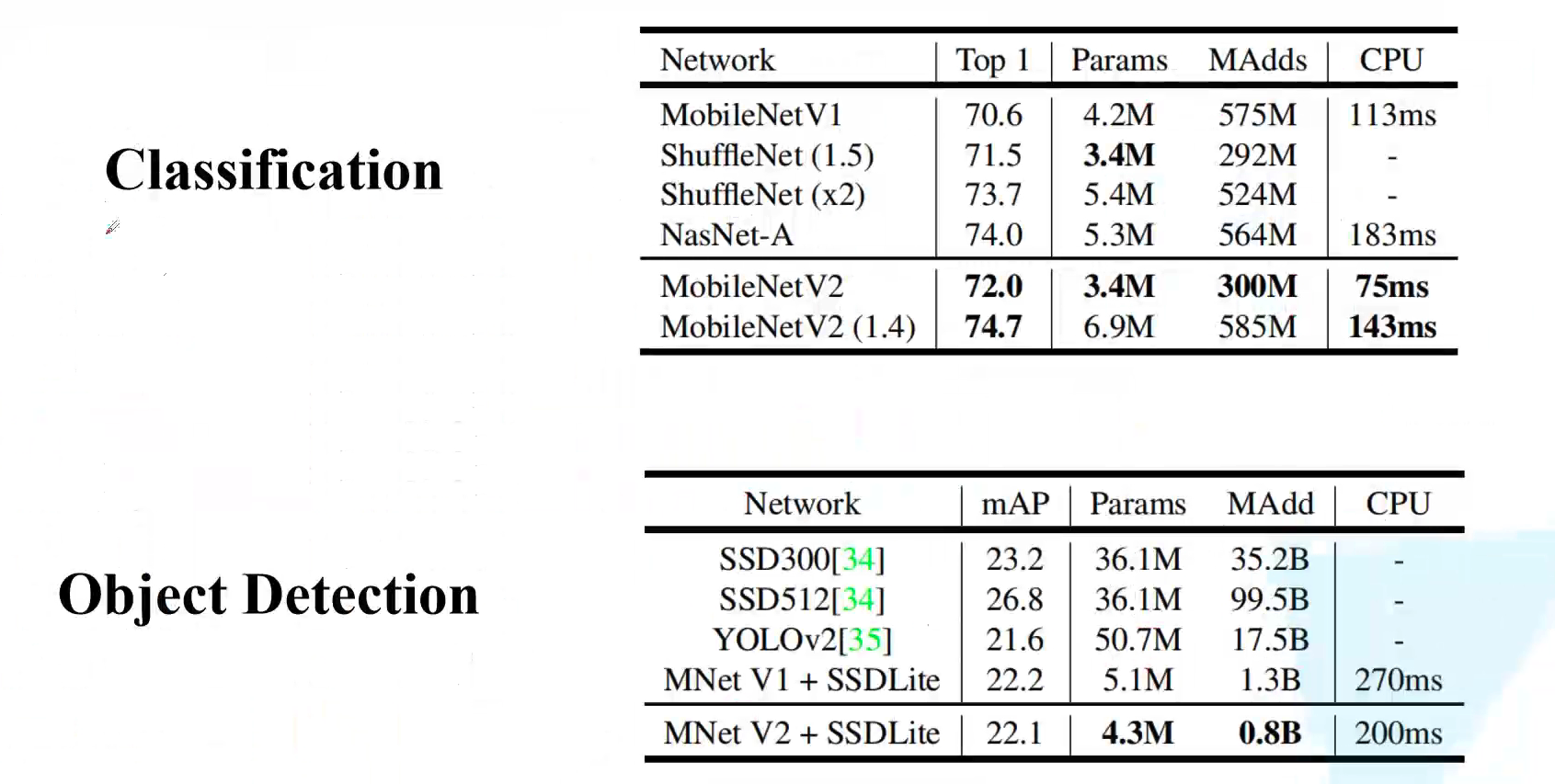
Let's take a look at the final performance comparison. Compared with MobileNetV1, it improves both parameter quantity and performance. It takes less than 0.1s to predict a graph on the CPU, which can be said to achieve real-time. However, the performance of target detection is slightly worse than that of MobileNetV1.

5. Code

The implementation code of MobileNetV2 is as follows:

from torch import nn
import torch


def _make_divisible(ch, divisor=8, min_ch=None):
    """
    This function is taken from the original tf repo.
    It ensures that all layers have a channel number that is divisible by 8
    It can be seen here:
    https://github.com/tensorflow/models/blob/master/research/slim/nets/mobilenet/mobilenet.py
    """
    if min_ch is None:
        min_ch = divisor
    new_ch = max(min_ch, int(ch + divisor / 2) // divisor * divisor)
    # Make sure that round down does not go down by more than 10%.
    if new_ch < 0.9 * ch:
        new_ch += divisor
    return new_ch


class ConvBNReLU(nn.Sequential):
    def __init__(self, in_channel, out_channel, kernel_size=3, stride=1, groups=1):
        padding = (kernel_size - 1) // 2
        super(ConvBNReLU, self).__init__(
            nn.Conv2d(in_channel, out_channel, kernel_size, stride, padding, groups=groups, bias=False),
            nn.BatchNorm2d(out_channel),
            nn.ReLU6(inplace=True)
        )


class InvertedResidual(nn.Module):
    def __init__(self, in_channel, out_channel, stride, expand_ratio):
        super(InvertedResidual, self).__init__()
        hidden_channel = in_channel * expand_ratio
        self.use_shortcut = stride == 1 and in_channel == out_channel

        layers = []
        if expand_ratio != 1:
            # 1x1 pointwise conv
            layers.append(ConvBNReLU(in_channel, hidden_channel, kernel_size=1))
        layers.extend([
            # 3x3 depthwise conv
            ConvBNReLU(hidden_channel, hidden_channel, stride=stride, groups=hidden_channel),
            # 1x1 pointwise conv(linear)
            nn.Conv2d(hidden_channel, out_channel, kernel_size=1, bias=False),
            nn.BatchNorm2d(out_channel),
        ])

        self.conv = nn.Sequential(*layers)

    def forward(self, x):
        if self.use_shortcut:
            return x + self.conv(x)
        else:
            return self.conv(x)


class MobileNetV2(nn.Module):
    def __init__(self, num_classes=1000, alpha=1.0, round_nearest=8):
        super(MobileNetV2, self).__init__()
        block = InvertedResidual
        input_channel = _make_divisible(32 * alpha, round_nearest)
        last_channel = _make_divisible(1280 * alpha, round_nearest)

        inverted_residual_setting = [
            # t, c, n, s
            [1, 16, 1, 1],
            [6, 24, 2, 2],
            [6, 32, 3, 2],
            [6, 64, 4, 2],
            [6, 96, 3, 1],
            [6, 160, 3, 2],
            [6, 320, 1, 1],
        ]

        features = []
        # conv1 layer
        features.append(ConvBNReLU(3, input_channel, stride=2))
        # building inverted residual residual blockes
        for t, c, n, s in inverted_residual_setting:
            output_channel = _make_divisible(c * alpha, round_nearest)
            for i in range(n):
                stride = s if i == 0 else 1
                features.append(block(input_channel, output_channel, stride, expand_ratio=t))
                input_channel = output_channel
        # building last several layers
        features.append(ConvBNReLU(input_channel, last_channel, 1))
        # combine feature layers
        self.features = nn.Sequential(*features)

        # building classifier
        self.avgpool = nn.AdaptiveAvgPool2d((1, 1))
        self.classifier = nn.Sequential(
            nn.Dropout(0.2),
            nn.Linear(last_channel, num_classes)
        )

        # weight initialization
        for m in self.modules():
            if isinstance(m, nn.Conv2d):
                nn.init.kaiming_normal_(m.weight, mode='fan_out')
                if m.bias is not None:
                    nn.init.zeros_(m.bias)
            elif isinstance(m, nn.BatchNorm2d):
                nn.init.ones_(m.weight)
                nn.init.zeros_(m.bias)
            elif isinstance(m, nn.Linear):
                nn.init.normal_(m.weight, 0, 0.01)
                nn.init.zeros_(m.bias)

    def forward(self, x):
        x = self.features(x)
        x = self.avgpool(x)
        x = torch.flatten(x, 1)
        x = self.classifier(x)
        return x