(3) Probability and information theory)
2, Linear algebra
Purpose: it is mainly to reduce the dimension of data and restore or build the target with the least data
2.1 eigenvalue decomposition
Only symmetric positive definite matrix can be decomposed into eigenvalues.
Eigenvalue decomposition: A = P * B * PT, where B is the diagonal matrix whose diagonal element is the eigenvalue of a, and P is the orthogonal matrix composed of the eigenvector of A.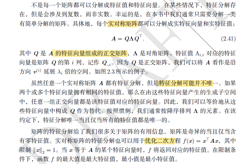
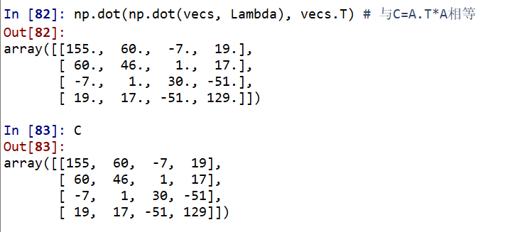
Then let's look at whether the row vector or column vector in vec decomposed by eig in np is an eigenvector.
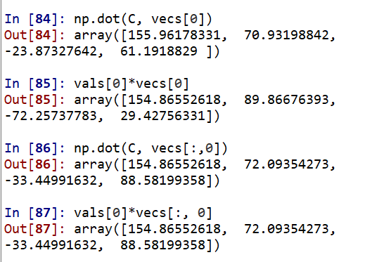
It can be seen that the latter is equal, indicating that the column vector of vecs decomposed by eig in np is an eigenvector.
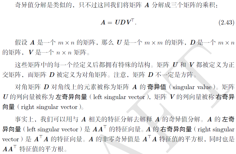
2.2 singular value decomposition
Every real matrix has a singular value decomposition, but not necessarily an eigendecomposition. For example, the matrix of non square matrix has no eigendecomposition, so we can only use singular value decomposition.
Examples and functions of singular value decomposition: https://www.cnblogs.com/pinard/p/6251584.html
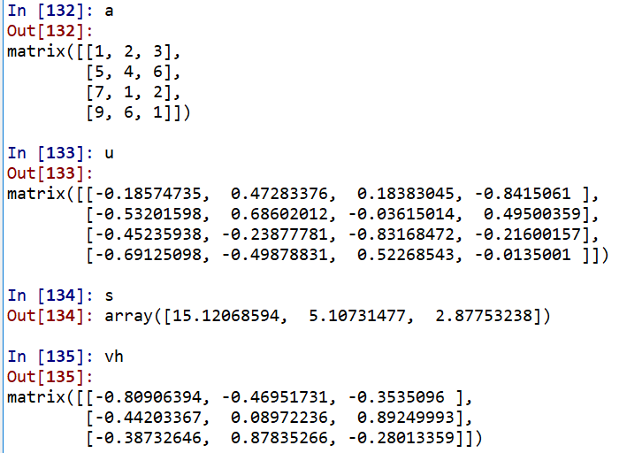
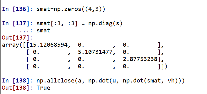
#2.1 eigenvalue decomposition
import numpy as np
from numpy.linalg import eig
A = np.random.randint(-10,10,(4,4))
A
C = np.dot(A.T, A)# Generating symmetric positive definite matrix
vals,vecs = eig(C)
vals
vecs
Lambda = np.diag(vals)#First, the eigenvalue is transformed into a matrix
np.dot(np.dot(vecs, Lambda), vecs.T) # Equal to C=A.T*A
#Then let's see whether the row vector or column vector in vec decomposed by eig in np is an eigenvector. Just verify: A*vecs[0] = vals[0]*vecs[0]
np.dot(C, vecs[0])
vals[0]*vecs[0]
np.dot(C, vecs[:,0])
vals[0]*vecs[:, 0]
#2.2 singular value decomposition
from numpy.linalg import svd
a = np.random.randint(-10,10,(4, 3)).astype(float)
u, s, vh = np.linalg.svd(a)# Here vh is the transpose of V
u.shape, s.shape, vh.shape
#Transform s into singular value matrix
smat=np.zeros((4,3))
smat[:3, :3] = np.diag(s)
smat
np.allclose(a, np.dot(u, np.dot(smat, vh)))
https://www.cnblogs.com/cymwill/p/9937850.html The above example follows this link. Finally, the singular value is transformed into a matrix error, which can only be re assigned into a 4 * 3 matrix.
2.3 Moore Penrose pseudoinverse
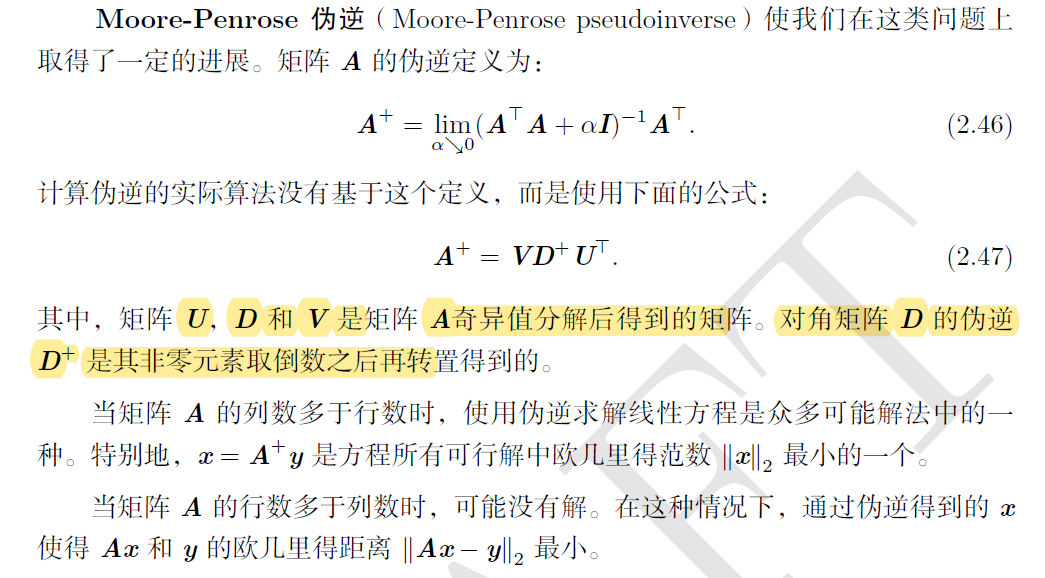
UDVT can be obtained by singular value decomposition, and the diagonal matrix D + is obtained by taking the reciprocal of the non-zero elements in D and then transposing. Examples and code references https://www.section.io/engineering-education/moore-penrose-pseudoinverse/ . Seems to be transposed directly in the link?
Note that in the previous SVD decomposition, a new blank row is created when converting Array D into matrix. In this link, a new blank column is created. The number of rows and columns of singular value matrix D is the same as that of the original matrix, and the number of rows and columns of matrix D + in violation is opposite to that of the original matrix.
If you calculate directly, call numpy linalg. Pinv() function.
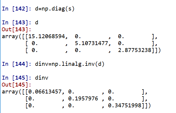
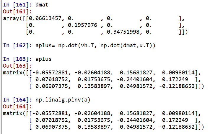
a=np.mat([[1,2,3],[5,4,6],[7,1,2],[9,6,1]])
u, s, vh = np.linalg.svd(a)# Here vh is the transpose of V, U,D,VT
d=np.diag(s)
dinv=np.linalg.inv(d)#Reciprocal of singular value diagonal matrix?
dmat=np.zeros((3,4))
dmat[:3, :3]=dinv#Unified into the number of rows and columns opposite to the original matrix
aplus= np.dot(vh.T, np.dot(dmat,u.T))
np.linalg.pinv(a)
2.4 PCA principal component analysis
https://zhuanlan.zhihu.com/p/37777074
While reducing the indicators to be analyzed, try to reduce the loss of information contained in the original indicators, so as to achieve the purpose of comprehensive analysis of the collected data.
The main idea of PCA is to map n-dimensional features to k-dimension, which is a new orthogonal feature, also known as the main component. It is a k-dimensional feature reconstructed from the original n-dimensional features.
The job of PCA is to find a set of mutually orthogonal coordinate axes from the original space. The selection of new coordinate axes is closely related to the data itself. Among them, the first new coordinate axis selection is the direction with the largest variance in the original data, the second new coordinate axis selection is the one with the largest variance in the plane orthogonal to the first coordinate axis, and the third axis is the one with the largest variance in the plane orthogonal to the first and second axes. By analogy, n such coordinate axes can be obtained. Through the new coordinate axes obtained in this way, we find that most of the variance is contained in the first k coordinate axes, and the variance of the latter coordinate axes is almost 0. Therefore, we can ignore the remaining coordinate axes and only keep the first k coordinate axes containing most of the variance. In fact, this is equivalent to retaining only the dimension features that contain most of the variance, while ignoring the feature dimensions that contain almost zero variance, so as to reduce the dimension of data features.
Think: how do we get these principal component directions that contain the greatest differences?
Answer: in fact, by calculating the covariance matrix of the data matrix, the eigenvalue eigenvector of the covariance matrix is obtained, and the matrix composed of the eigenvectors corresponding to the k features with the largest eigenvalue (i.e. the largest variance) is selected. In this way, the data matrix can be transformed into a new space to reduce the dimension of data features. There are two solutions: eigenvalue decomposition covariance matrix and singular value decomposition covariance matrix.
One problem of PCA algorithm is that it is not interpretable
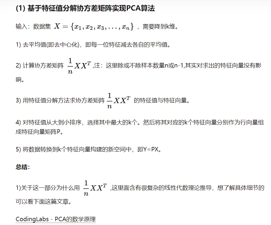
2.4.1 eigenvalue decomposition covariance matrix
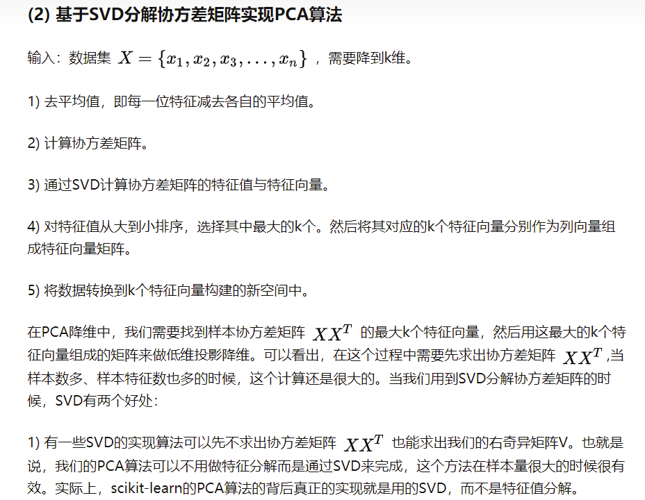
2.4.2 singular value decomposition
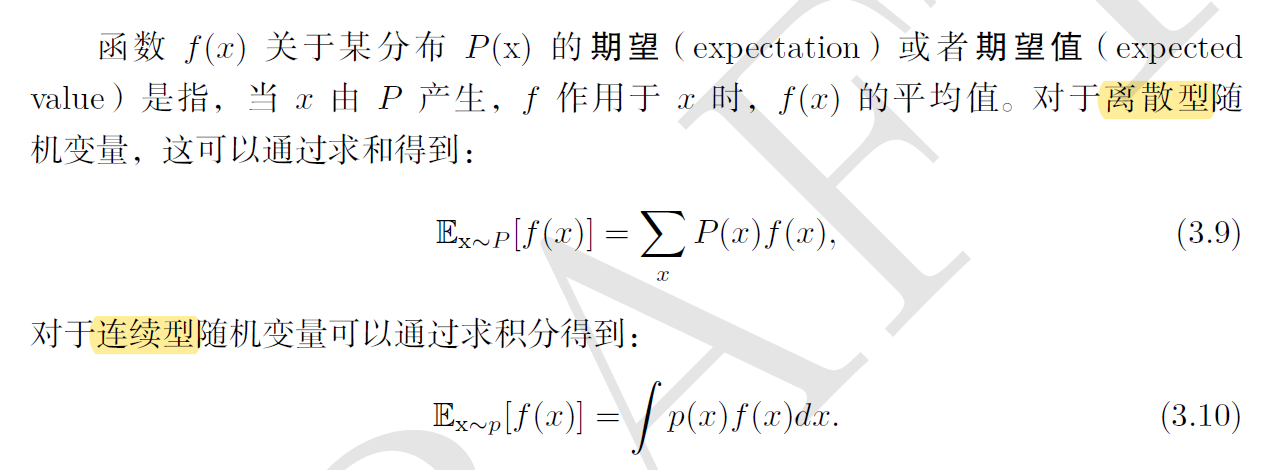
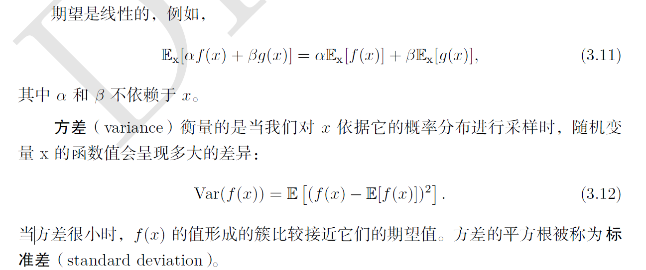
3, Probability and information theory
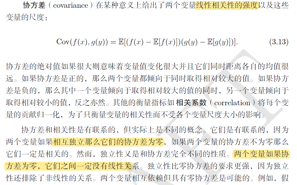
3.1 expected variance covariance
The covariance of the two variables is 0, indicating that they are not related, there must be no linear relationship, and they may not be independent; If the two variables are independent, the covariance must be 0 and there is no correlation.
Common probability distribution
https://blog.csdn.net/qq_27388259/article/details/112168913
3.2.1 common probability distribution in probability theory
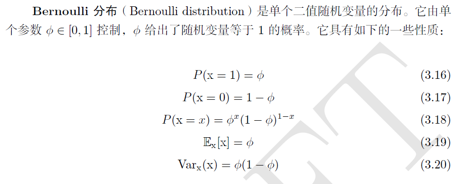
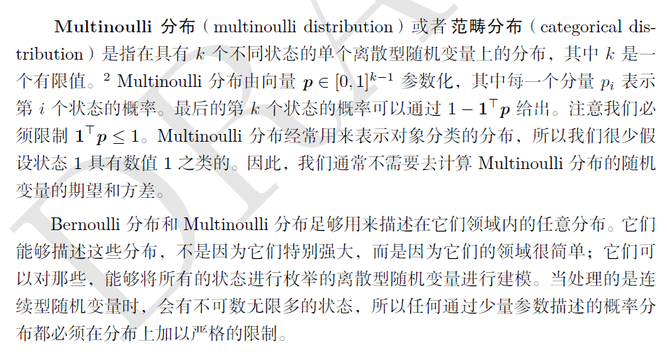
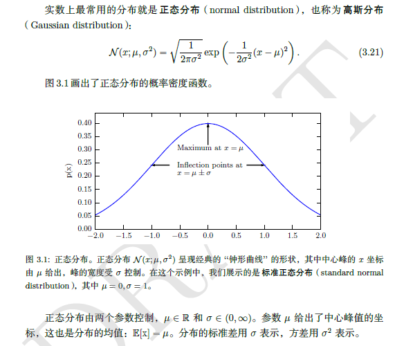
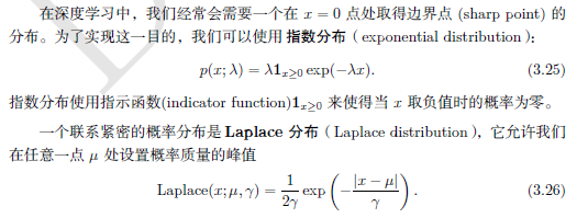
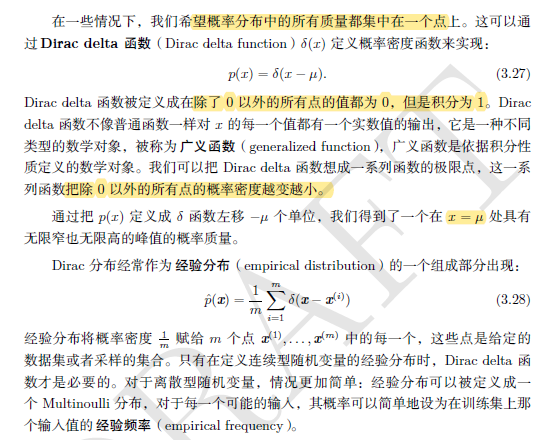
3.2.2 common probability distribution in deep learning
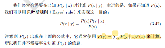
3.2.3 Bayesian rules
Finally have their own original code.
import pandas as pd
import numpy as np
#data=pd.DataFrame(columns=('x1','x2','x3','y'))
data=[['yes','single','high','no'],
      ['no','married','middle','no'],
      ['no','single','low','no'],
      ['yes','married','middle','no'],
      ['no','divorced','middle','yes'],
      ['no','married','low','no'],
      ['yes','divorced','high','no'],
      ['no','single','low','yes'],
      ['no','married','low','no'],
      ['no','single','low','yes']]

#Find the individual a priori probability p(x|y)
def naivebayes(data,n,x,y):#n is the nth column, x is the value classified as x in the nth column, and y is the label item
   numEntires = len(data)                        #Returns the number of rows in the dataset
   labelCounts = {} #y
   for featVec in data:
        currentLabel = featVec[-1]
        if currentLabel not in labelCounts.keys():
            labelCounts[currentLabel] = 0
        labelCounts[currentLabel] += 1
   num=0
   for i in range(len(data)):
        if data[i][-1] == y and data[i][n] == x:
             num = num + 1
   #print (num/labelCounts[y])
   print ('p(',y,')The probability is:',labelCounts[y]/numEntires)#p(y)
   return (num/labelCounts[y])#p(x|y)

p1=naivebayes(data,0,'no','no')
print(p1)
p2=naivebayes(data,1,'divorced','no')
print(p2)
p3=naivebayes(data,2,'low','no')
print(p3)
#Find p(y|x) = multiply individual p and * p(y)
print(p1*p2*p3)
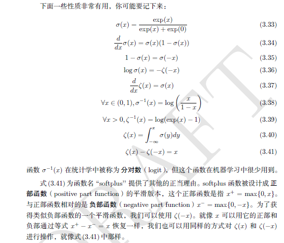
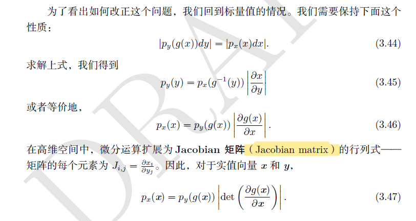
3.2.4 technical details of continuous variables
3.3 information theory
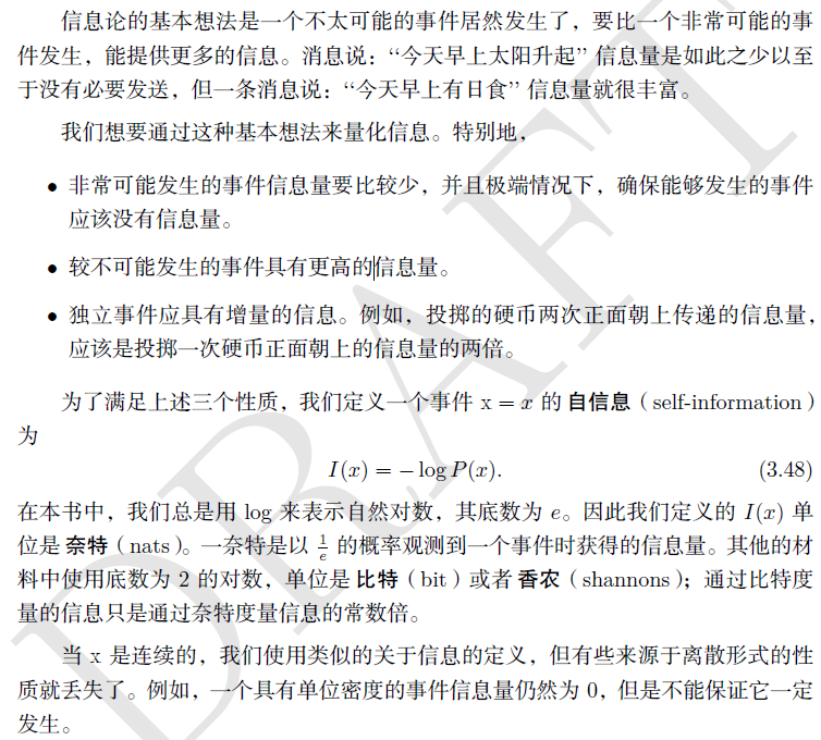
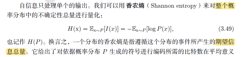
3.3.1 information quantity: self information and Shannon entropy
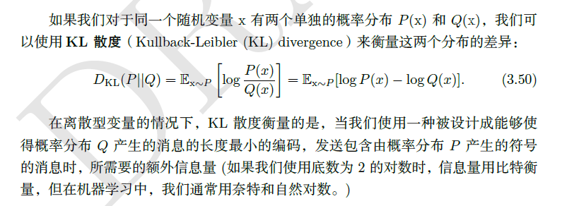
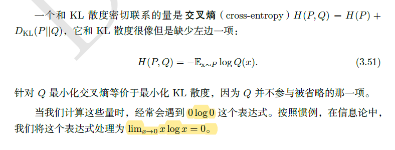
3.3.2 DKL divergence and cross entropy H(P,Q)
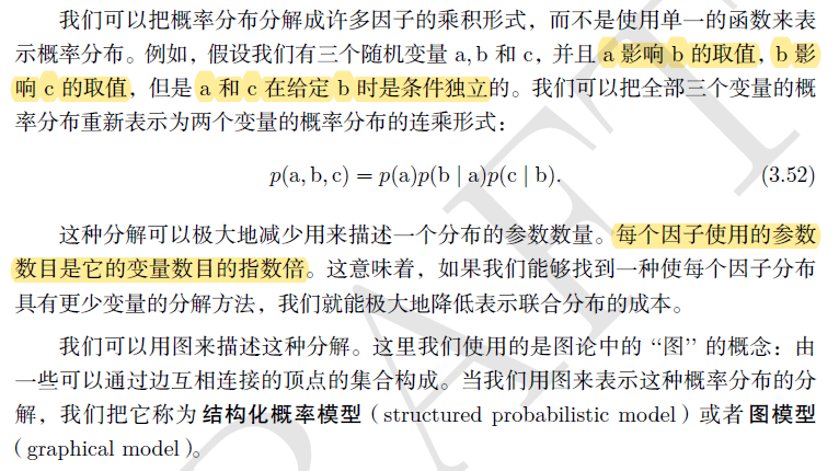
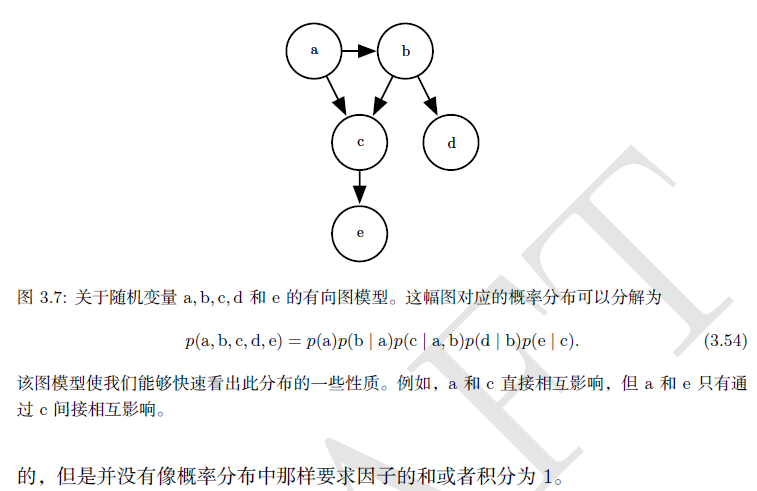
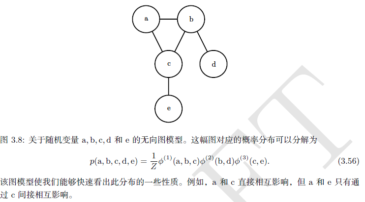
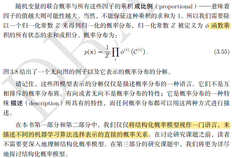
3.5 structured probability model