Prepare 1: OpenCV Common Picture Conversion Skills
Before computer vision model training, we often use image enhancement techniques to obtain more samples, but some methods in depth learning framework may not meet our needs for image transformation, so we still have a lot of common image processing techniques in OpenCV. Help.
Image Channel Separation
We know that each image is composed of three RGB color channels, so we can use split function to separate the three channels of the original image.
B, G, R = cv2.split(img)
After channel separation, we can perform numerical transformation independently on each channel, and then combine the transformation to generate new images, such as enhancing the brightness of the image:
B,G,R = cv2.split(img)
for i in (B,G,R):
    randint = random.randint(50,100)
    limit = 255-randint
    i[i>limit]=255
    i[i<=limit]=randint+i[i<=limit]
img_merge = cv2.merge((B,G,R))
cv2.imshow("img_merge",img_merge)
key = cv2.waitKey()
if key==27:
    cv2.destroyAllWindows()
Image rotation
The warpAffine function can also be used to rotate the image according to the angle we set:
M = cv2.getRotationMatrix2D((img.shape[1] / 2, img.shape[0] / 2), 30, 1)
img_rotate = cv2.warpAffine(img, M, (img.shape[1], img.shape[0]))

cv2.imshow('img_rotate', img_rotate)
key = cv2.waitKey(0)
if key == 27:
    cv2.destroyAllWindows()
Here we don't zoom in and rotate the image at 30 degrees.
affine transformation
Affine transformation allows image tilting and scaling in any two directions. The code is as follows:
def random_warp(img, row, col):
    height, width, channels = img.shape

    random_margin = 100
    x1 = random.randint(-random_margin, random_margin)
    y1 = random.randint(-random_margin, random_margin)
    x2 = random.randint(width - random_margin - 1, width - 1)
    y2 = random.randint(-random_margin, random_margin)
    x3 = random.randint(width - random_margin - 1, width - 1)
    y3 = random.randint(height - random_margin - 1, height - 1)
    x4 = random.randint(-random_margin, random_margin)
    y4 = random.randint(height - random_margin - 1, height - 1)

    dx1 = random.randint(-random_margin, random_margin)
    dy1 = random.randint(-random_margin, random_margin)
    dx2 = random.randint(width - random_margin - 1, width - 1)
    dy2 = random.randint(-random_margin, random_margin)
    dx3 = random.randint(width - random_margin - 1, width - 1)
    dy3 = random.randint(height - random_margin - 1, height - 1)
    dx4 = random.randint(-random_margin, random_margin)
    dy4 = random.randint(height - random_margin - 1, height - 1)

    pts1 = np.float32([[x1, y1], [x2, y2], [x3, y3], [x4, y4]])
    pts2 = np.float32([[dx1, dy1], [dx2, dy2], [dx3, dy3], [dx4, dy4]])


    M_warp = cv2.getPerspectiveTransform(pts1, pts2)
    img_warp = cv2.warpPerspective(img, M_warp, (width, height))
    return img_warp

img_warp = random_warp(img, img.shape[0], img.shape[1])

cv2.imshow('img_warp', img_warp)
key = cv2.waitKey(0)
if key == 27:
    cv2.destroyAllWindows()
Gamma Correction
Gamma correction improves the contrast of the image and makes it look brighter. The code is as follows:
def adjust_gamma(image, gamma=1.0):
    invGamma = 1.0/gamma
    table = []
    for i in range(256):
        table.append(((i / 255.0) ** invGamma) * 255)
    table = np.array(table).astype("uint8")
    return cv2.LUT(image, table)

img_gamma = adjust_gamma(img, 2)
cv2.imshow("img",img)
cv2.imshow("img_gamma",img_gamma)

key = cv2.waitKey()
if key == 27:
    cv2.destroyAllWindows()
Prepare 2: Download and install cv2
Download the wheel as follows:

Then use the pip command directly:
pip install opencv_python-3.4.3-cp37-cp37m-win_amd64.whl
Note: OpenCV for Python is now bound through Numpy. So we must master some knowledge of Numpy when we use it! Images are matrices. In OpenCV for Python, images are arrays in Numpy!
1. Image loading, display and storage
If you read an image, you only need imread.
import cv2

# Get pictures
img_path = r'1.jpg'
img = cv2.imread(img_path)
OpenCV currently supports reading common formats such as bmp, jpg, png, tiff, etc.
We can also look at some basic properties of the image:
print(img)
print(img.dtype)
print(img.shape)
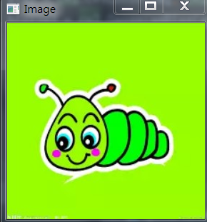
Next, create a window
cv2.namedWindow("Image")
Then display the image in the window
cv2.imshow('Image', img)
Finally, add one more sentence:
cv2.waitKey(0)
If the last sentence is not added, the execution window in IDLE will not respond directly. When executed on the command line, it flashes by.
It's easy to save images, just cv.imwrite.
cv2.imwrite(save_path, crop_img)
The first parameter is the saved path and file name, and the second is the image matrix. Among them, imwrite() has an optional third parameter, as follows:
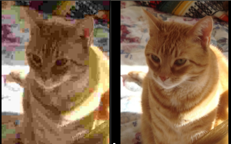
cv2.imwrite("cat.jpg", img,[int(cv2.IMWRITE_JPEG_QUALITY), 5])
The third parameter is for a specific format: for JPEG, it represents the quality of the image, expressed as an integer of 0-100, which defaults to 95. Note that the cv2.IMWRITE_JPEG_QUALITY type is Long and must be converted to int. Below are two pictures stored in different quality:
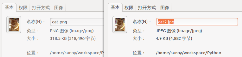
For PNG, the third parameter represents the compression level. cv2.IMWRITE_PNG_COMPRESSION, from 0 to 9, the higher the compression level, the smaller the image size. The default level is 3:
cv2.imwrite("./cat.png", img, [int(cv2.IMWRITE_PNG_COMPRESSION), 0])

cv2.imwrite("./cat2.png", img, [int(cv2.IMWRITE_PNG_COMPRESSION), 9])
The size of the saved image is as follows:
There is also a supporting image, which is not commonly used.
The complete procedure is as follows:
#!/usr/bin/env python
# -*- coding: utf-8 -*-
import cv2

# Get pictures
img_path = r'1.jpg'
img = cv2.imread(img_path)
cv2.namedWindow("Image")
cv2.imshow('Image', img)
cv2.waitKey(0)
cv2.destroyAllWindows()
It's a good habit to finally release the window! View the picture as follows:
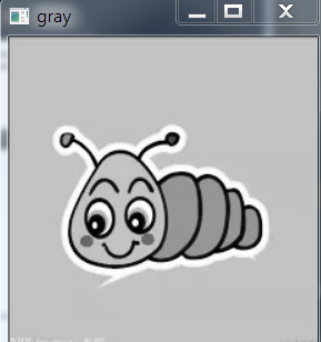
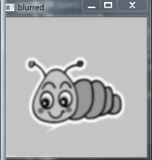
2. Conversion of gray level and de-noising
We can get two pictures, the first one is gray scale image, and the second one is after denoising. There are many methods of denoising, such as mean filter, Gauss filter, median filter, bilateral filter, etc. Here we show the grayscale, Gaussian denoising code:
gray = cv2.cvtColor(img, cv2.COLOR_BGR2GRAY)

blurred = cv2.GaussianBlur(gray, (9, 9),0)
The image below shows the effect. (Gauss is chosen here because Gauss denoising is the best.)
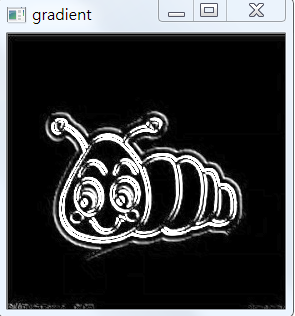
3. Extracting Gradient of Image
Sobel operator is used to calculate the gradient in x and y direction, and then the gradient in minus y direction in x direction. Through this operation, the image region with high horizontal gradient and low vertical gradient will be left.
The code goes as follows:
# Gradient extraction of image
gradX = cv2.Sobel(gray, ddepth=cv2.CV_32F, dx=1, dy=0)
gradY = cv2.Sobel(gray, ddepth=cv2.CV_32F, dx=0, dy=1)

gradient = cv2.subtract(gradX, gradY)
gradient = cv2.convertScaleAbs(gradient)
At this point we will get the following images:
4. Continue de-noising
Considering the pore of the image, the low-pass filter is used to smooth the image first, which will help to smooth the high-frequency noise in the image. The purpose of low-pass filter is to reduce the change rate of image.
If each pixel is replaced by the mean of the pixels around the image, it can smooth and replace those areas with obvious intensity changes.
For binarization of blurred images, as the name implies, image values are divided into two kinds of values with a certain boundary:
blurred = cv2.GaussianBlur(gradient, (9, 9), 0)

(_, thresh) = cv2.threshold(blurred, 90, 255, cv2.THRESH_BINARY)
The effect is as follows:
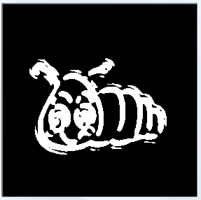
In fact, even if we do manual segmentation, we still need to find a boundary, we can see the outline, but we ultimately want the whole outline, so the internal small area is not.
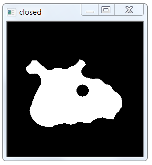
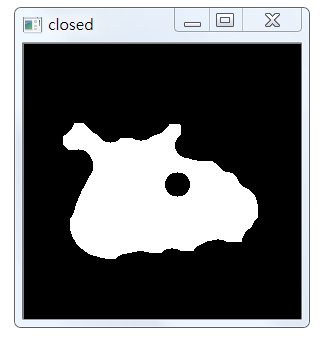
5. Image Morphology
Here we select ELLIPSE core and use CLOSE operation.
# Image Morphology
kernel = cv2.getStructuringElement(cv2.MORPH_ELLIPSE, (25, 25))

closed = cv2.morphologyEx(thresh, cv2.MORPH_CLOSE, kernel)
At this time, the effect is as follows:
6. Details
Comparing with the original image, we can find that there is a loss of detail, which will interfere with the detection of insect contour. We need to expand the insect contour and perform four morphological corrosion and expansion respectively. The code is as follows:
# Detailed description, four times morphological corrosion and expansion respectively
closed = cv2.erode(closed, None, iterations=4)

closed = cv2.dilate(closed, None, iterations=4)
The results are as follows:
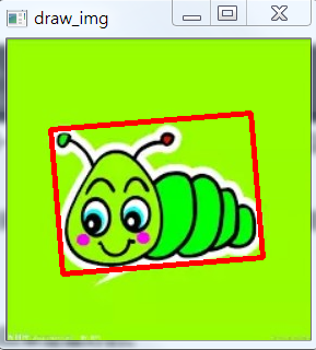
7. Find out the outline of the insect area and draw it.
In this case, the cv2.findContours() function is used as follows:
(_, cnts, _) = cv2.findContours(
   //PARAMETER 1: BINARY IMAGE
   closed.copy(),
   //Parametric 2: Contour type
   #Represents that only outlines are detected
   # cv2.RETR_EXTERNAL,
   #Establish two levels of contour, with the upper level being the boundary.
   # cv2.RETR_CCOMP,
   #Detection contours do not establish hierarchical relationships
   # cv2.RETR_LIST,
   #Establishing the outline of a hierarchical tree structure
   # cv2.RETR_TREE,
   #Store all contour points, and the difference of pixel position between two adjacent points is no more than 1.
   # cv2.CHAIN_APPROX_NONE,
   //PARAMETER 3: PROCESSING APPROXIMATION METHOD
   #For example, a rectangular contour only needs four points to store contour information.
   # cv2.CHAIN_APPROX_SIMPLE,
   # cv2.CHAIN_APPROX_TC89_L1,
   # cv2.CHAIN_APPROX_TC89_KCOS
   )
The first parameter is the image to be retrieved, which must be a binary image, i.e. a black-and-white (not a gray-scale image).
# Here, opencv3 returns three parameters
(_, cnts, _) = cv2.findContours(
    # PARAMETER 1: BINARY IMAGE
    closed.copy(),
    # Parametric 2: Contour type
    cv2.RETR_LIST,
    cv2.CHAIN_APPROX_SIMPLE
)
c = sorted(cnts, key=cv2.contourArea, reverse=True)[0]
rect = cv2.minAreaRect(c)
box = np.int0(cv2.boxPoints(rect))

draw_img = cv2.drawContours(img.copy(), [box], -1, (0, 0, 255), 3)
cv2.imshow("draw_img", draw_img)
At this point, you will get:
8. Cutting
The simplest way to crop an image is to obtain slices of an array of images, as follows:
img_crop = img[100:300,100:300]
cv2.imshow("img_crop", img_crop)
key = cv2.waitKey()
if key == 27:
    cv2.destroyAllWindows()
Of course, here we find four points directly, cut them out on OK.
In fact, the coordinates of the four vertices in the green matrix region are stored in the box. We tailor the insect image as shown in the figure below.
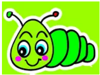
The method is to find the maximum and minimum x and y coordinates of four vertices. The new image is higher than max(Y) - min(Y), and its width is equal to max(X) - min(X).
Xs = [i[0] for i in box]
Ys = [i[1] for i in box]
x1 = min(Xs)
x2 = max(Xs)
y1 = min(Ys)
y2 = max(Ys)
hight = y2 - y1
width = x2 - x1
crop_img= img[y1:y1+hight, x1:x1+width]
cv2.imshow('crop_img', crop_img)
9. Complete code
#-*- coding: UTF-8 -*-
import cv2
import numpy as np


def get_image(path):
   #Get pictures
   img=cv2.imread(path)
   gray=cv2.cvtColor(img,cv2.COLOR_BGR2GRAY)

   return img, gray

def Gaussian_Blur(gray):
   # Gauss denoising
   blurred = cv2.GaussianBlur(gray, (9, 9),0)

   return blurred

def Sobel_gradient(blurred):
   # Computation of x and y direction gradient by Sorber operator
   gradX = cv2.Sobel(blurred, ddepth=cv2.CV_32F, dx=1, dy=0)
   gradY = cv2.Sobel(blurred, ddepth=cv2.CV_32F, dx=0, dy=1)

   gradient = cv2.subtract(gradX, gradY)
   gradient = cv2.convertScaleAbs(gradient)

   return gradX, gradY, gradient

def Thresh_and_blur(gradient):

   blurred = cv2.GaussianBlur(gradient, (9, 9),0)
   (_, thresh) = cv2.threshold(blurred, 90, 255, cv2.THRESH_BINARY)

   return thresh

def image_morphology(thresh):
   # Establishing an Elliptic Kernel Function
   kernel = cv2.getStructuringElement(cv2.MORPH_ELLIPSE, (25, 25))
   # Executing image morphology, looking up documents directly in detail, is very simple.
   closed = cv2.morphologyEx(thresh, cv2.MORPH_CLOSE, kernel)
   closed = cv2.erode(closed, None, iterations=4)
   closed = cv2.dilate(closed, None, iterations=4)

   return closed

def findcnts_and_box_point(closed):
   # Here, opencv3 returns three parameters
   (_, cnts, _) = cv2.findContours(closed.copy(),
       cv2.RETR_LIST,
       cv2.CHAIN_APPROX_SIMPLE)
   c = sorted(cnts, key=cv2.contourArea, reverse=True)[0]
   # compute the rotated bounding box of the largest contour
   rect = cv2.minAreaRect(c)
   box = np.int0(cv2.boxPoints(rect))

   return box

def drawcnts_and_cut(original_img, box):
   # Because this function is very destructive, all of them need to be drawn on img.copy().
   # draw a bounding box arounded the detected barcode and display the image
   draw_img = cv2.drawContours(original_img.copy(), [box], -1, (0, 0, 255), 3)

   Xs = [i[0] for i in box]
   Ys = [i[1] for i in box]
   x1 = min(Xs)
   x2 = max(Xs)
   y1 = min(Ys)
   y2 = max(Ys)
   hight = y2 - y1
   width = x2 - x1
   crop_img = original_img[y1:y1+hight, x1:x1+width]

   return draw_img, crop_img

def walk():

   img_path = r'C:\Users\aixin\Desktop\chongzi.png'
   save_path = r'C:\Users\aixin\Desktop\chongzi_save.png'
   original_img, gray = get_image(img_path)
   blurred = Gaussian_Blur(gray)
   gradX, gradY, gradient = Sobel_gradient(blurred)
   thresh = Thresh_and_blur(gradient)
   closed = image_morphology(thresh)
   box = findcnts_and_box_point(closed)
   draw_img, crop_img = drawcnts_and_cut(original_img,box)

   # Be violent. Show them all.

   cv2.imshow('original_img', original_img)
   cv2.imshow('blurred', blurred)
   cv2.imshow('gradX', gradX)
   cv2.imshow('gradY', gradY)
   cv2.imshow('final', gradient)
   cv2.imshow('thresh', thresh)
   cv2.imshow('closed', closed)
   cv2.imshow('draw_img', draw_img)
   cv2.imshow('crop_img', crop_img)
   cv2.waitKey(20171219)
   cv2.imwrite(save_path, crop_img)

walk()
Appendix code:
# Used to transform image formats
img = cv2.cvtColor(src,
   COLOR_BGR2HSV # BGR---->HSV
   COLOR_HSV2BGR # HSV---->BGR
   ...)
# For HSV, Hue range is [0,179], Saturation range is [0,255] and Value range is [0,255]


# Returns a threshold, and a binary image. The first threshold is used for the otsu method.
# But not now, because it can be implemented directly through mahotas
T = ret = mahotas.threshold(blurred)
ret, thresh_img = cv2.threshold(src, # Generally, gray image
   num1, # Image threshold
   num2, # If it is greater than or num1, the pixel value will become num2
# The last binarization parameter
   cv2.THRESH_BINARY      # Set the gray value greater than the threshold to the maximum gray value and the value less than the threshold to 0.
   cv2.THRESH_BINARY_INV  # Set the gray value greater than the threshold to 0, and the value greater than the threshold to the maximum gray value.
   cv2.THRESH_TRUNC       # Set the gray value larger than the threshold value as the threshold value, and keep the value smaller than the threshold value unchanged.
   cv2.THRESH_TOZERO      # Set the gray value less than the threshold to 0, and the value greater than the threshold remains unchanged.
   cv2.THRESH_TOZERO_INV  # Set the gray value above the threshold to 0, and keep the value below the threshold unchanged.
)
thresh = cv2.AdaptiveThreshold(src,
   dst,
   maxValue,
   # adaptive_method
   ADAPTIVE_THRESH_MEAN_C,
   ADAPTIVE_THRESH_GAUSSIAN_C,
   # thresholdType
   THRESH_BINARY,
   THRESH_BINARY_INV,
   blockSize=3,
   param1=5
)


# Usually white objects are found in black background, so the original image background is preferably black.
# When performing edge finding, it is usually done after threshold or canny edge detection.
# warning: This function modifies the original image.
# Return: coordinate position (x,y),
(_, cnts, _) = cv2.findContours(mask.copy(),
   # cv2.RETR_EXTERNAL,             #Represents that only outlines are detected
   # cv2.RETR_CCOMP,                #Establish two levels of contour, with the upper level being the boundary.
   cv2.RETR_LIST,                 #Detection contours do not establish hierarchical relationships
   # cv2.RETR_TREE,                   #Establishing the outline of a hierarchical tree structure
   # cv2.CHAIN_APPROX_NONE,           #Store all contour points, and the difference of pixel position between two adjacent points is no more than 1.
   cv2.CHAIN_APPROX_SIMPLE,       #For example, a rectangular contour only needs four points to store contour information.
   # cv2.CHAIN_APPROX_TC89_L1,
   # cv2.CHAIN_APPROX_TC89_KCOS
  )
img = cv2.drawContours(src, cnts, whichToDraw(-1), color, line)


img = cv2.imwrite(filename, dst,  # File Path, and Target Image File Matrix

   # For JPEG, the quality of the image is represented by an integer of 0-100, which defaults to 95.
   # Note that the cv2.IMWRITE_JPEG_QUALITY type is Long and must be converted to int
   [int(cv2.IMWRITE_JPEG_QUALITY), 5]
   [int(cv2.IMWRITE_JPEG_QUALITY), 95]
   # From 0 to 9, the higher the compression level, the smaller the image size. The default level is 3
   [int(cv2.IMWRITE_PNG_COMPRESSION), 5])
   [int(cv2.IMWRITE_PNG_COMPRESSION), 9])

# If you don't know which flags to use, after all, there's too much to remember, just look for them.
//Find a function or variable
events = [i for i in dir(cv2) if 'PNG' in i]
print( events )

//Find flags at the beginning of a variable
flags = [i for i in dir(cv2) if i.startswith('COLOR_')]
print flags

//Batch read file name
import os
filename_rgb = r'C:\Users\aixin\Desktop\all_my_learning\colony\20170629'
for filename in os.listdir(filename_rgb):              #The parameter of listdir is the path of the folder
   print (filename)
References: