Deep learning pytoch (IV) -- image classifier
1, Introduction
Typically, when processing image, text, voice, or video data, you can use standard Python to load the data into the numpy array format, and then convert the array to torch.*Tensor
- For images, you can use pilot and OpenCV
- For voice, you can use scipy, librosa
- For text, you can directly use Python or Python basic data to load modules, or NLTK and SpaCy
Especially for vision, pytoch has created a package called torchvision, which includes a data loading module torchvision.datasets that supports loading public data sets such as Imagenet, CIFAR10 and MNIST, and a data conversion module torch.utils.data.DataLoader that supports loading image data. This provides great convenience and avoids writing "boilerplate code"
2, Data set
For this section, CIFAR10 dataset is used, which contains three categories: aircraft, automobile, bird, cat, deer, dog, frog, horse, ship and truck. The image size in CIFAR10 is 33232, that is, the three-layer color channel of RGB, and the size in each layer channel is 32 * 32
3, Training an image classifier
Steps of training image classifier:
- The training and test data sets of CIFAR10 were loaded and normalized using torchvision
- A convolutional neural network is defined
- Define a loss function
- Training network on training sample data
- Test the network on the test sample data
1. Import the package
# Using torchvision, load and normalize CIFAR10
import torch
import torchvision
import torchvision.transforms as transforms
2. Normalization + labeling
# The output of torchvision dataset is PILImage with the range of [0,1], which is converted into Tensor tensor with the normalized range of [- 1,1]
transform=transforms.Compose(
    [transforms.ToTensor(),
     transforms.Normalize((0.5,0.5,0.5),(0.5,0.5,0.5))]
    )
# Training set
trainset=torchvision.datasets.CIFAR10(root='./data',train=True,download=False,transform=transform)
trainloader=torch.utils.data.DataLoader(trainset,batch_size=4,shuffle=True,num_workers=2)
# Test set
testset=torchvision.datasets.CIFAR10(root='./data',train=False,download=False,transform=transform)
testloader=torch.utils.data.DataLoader(testset,batch_size=4,shuffle=False,num_workers=2)

classes=("plane","car","bird","cat","deer","dog","frog","horse","ship","truck")
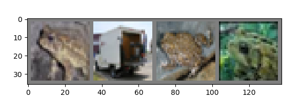
3. Let's start with the photos from Kangkang training center
# Show the training photos
import matplotlib.pyplot as plt
import numpy as np
# Define the function of picture display
def imshow(img):
img=img/2+0.5
npimg=img.numpy()
plt.imshow(np.transpose(npimg,(1,2,0)))
plt.show()
# Random training images are obtained
dataiter=iter(trainloader)
images,labels=dataiter.next()
# Show pictures
imshow(torchvision.utils.make_grid(images))
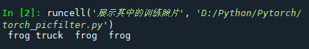
#Print labels labels
print(' '.join("%5s"%classes[labels[j]] for j in range(4)))
Operation results
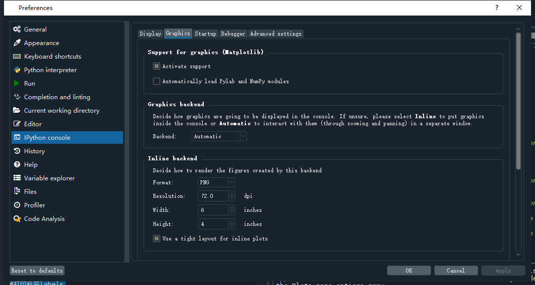
Note: for beginners, if Spyder does not display pictures, you can set them yourself. In Tools - > preferences, the settings are as follows:
4. Define a neural network
Here, copy the neural network in the previous section( ad locum ), and modify it to a 3-channel picture (previously defined as 1-channel)
#%%
# Define convolutional neural network
import torch.nn as nn
import torch.nn.functional as F

class Net(nn.Module):

    def __init__(self):
        super(Net,self).__init__()
        # 1 input, 6 outputs, 5 * 5 convolution
        # kernel
        self.conv1=nn.Conv2d(3,6,5)#Define three channels
        self.pool=nn.MaxPool2d(2,2)
        self.conv2=nn.Conv2d(6,16,5)
        # Mapping function: linear -- y=Wx+b
        self.fc1=nn.Linear(16*5*5,120)#Input characteristic value: 16 * 5 * 5, output characteristic value: 120
        self.fc2=nn.Linear(120,84)
        self.fc3=nn.Linear(84,10)

    def forward(self,x):
        x=self.pool(F.relu(self.conv1(x)))
        x=self.pool(F.relu(self.conv2(x)))
        x=x.view(-1,16*5*5)
        x=F.relu(self.fc1(x))
        x=F.relu(self.fc2(x))
        x=self.fc3(x)
        return x

net=Net()
Tips: in Spyder, you can use "#%%" to get cell blocks, and then run each cell. The shortcut key (Ctrl+Enter) - > I love to use shortcut keys. No matter what you can use the keyboard, you don't use the mouse (it's really lazy!!!)
5. Define a loss function and optimizer
The classification cross entropy cross entropy is used as the loss function and the momentum SGD is used as the optimizer
#%%
# Define a loss function and optimizer
import torch.optim as optim
criterion=nn.CrossEntropyLoss()
optimizer=optim.SGD(net.parameters(), lr=0.001,momentum=0.9)
6. Train the network
Here, you only need to loop the input network and optimizer on the data iterator
#%%Training network
for epoch in range(2):
running_loss=0.0
for i,data in enumerate(trainloader,0):
#Get input
inputs,labels=data
# Set the gradient value of the parameter to zero
optimizer.zero_grad()
#Back propagation + optimization
outputs=net(inputs)
loss=criterion(outputs,labels)
loss.backward()
optimizer.step()
#print data
running_loss+=loss.item()
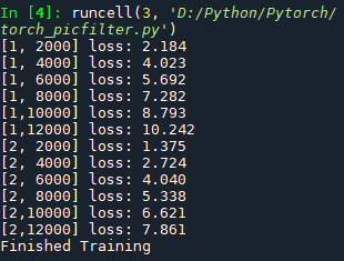
if i% 2000==1999:
print('[%d,%5d] loss: %.3f'%(epoch+1,i+1,running_loss/2000))#Every 2000 outputs
print('Finished Training')
Operation results
7. Test the network on the test set
The network has been trained twice through the training data set, but we need to check whether we have learned anything. The output of the neural network will be used as the prediction class mark to check the prediction performance of the network, and the real class mark of the sample will be used to check. If the prediction is correct, the sample will be added to the list of correct prediction
#%%
#Show on test set
outputs=net(images)
# The output is to predict the similarity with ten classes. The higher the similarity with a class, the more the network considers that the image belongs to this class
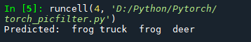
# Print the most similar category
_, predictd=torch.max(outputs,1)
print('Predicted:',' '.join('%5s'% classes[predictd[j]]
for j in range(4)))
Operation results
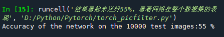
Put the network on the whole data set to see the specific performance
#%%The result looks good 55%. Look at the performance of the network in the whole data set
correct=0
total=0
with torch.no_grad():
    for data in testloader:
        images,labels=data
        outputs=net(images)
        _, predicted = torch.max(outputs.data, 1)
        total += labels.size(0)
        correct += (predicted==labels).sum().item()
print('Accuracy of the network on the 10000 test images:%d %%' % (
    100*correct/total))
Operation results
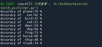
8. Check the training effect separately
#%%Category view
class_correct=list(0. for i in range(10))
class_total=list(0. for i in range(10))
with torch.no_grad():
    for data in testloader:
        images,labels=data
        outputs=net(images)
        _, predictd=torch.max(outputs,1)
        c=(predictd==labels).squeeze()
        for i in range(4):
            label=labels[i]
            class_correct[label]+=c[i].item()
            class_total[label]+=1


for i in range(10):
    print('Accuracy of %5s:%2d %%'% (classes[i],100*class_correct[i]/class_total[i]))
Operation results
Today is over, see you tomorrow! (wait, I have a class tomorrow morning. I don't know if I'm free. I'll try to see you! Hee hee)