This blog is only used to record the learning process, avoid forgetting and facilitate future review

Convolutional neural network is good at image processing. It is inspired by human visual nervous system.
CNN has two characteristics:
1. It can effectively reduce the dimension of pictures with large amount of data into small amount of data
2. It can effectively retain the image features, in line with the principle of image processing
At present, CNN has been widely used in many fields, such as face recognition, automatic driving, Meitu show, security and so on.

What problem did CNN solve

Before CNN appeared, we mainly encountered the following two problems in image processing:
1. The amount of data is too large, which makes the processing cost high and the efficiency low.
2. It is difficult to retain the original features of the image in the process of digitization, resulting in the low accuracy of image processing
The following two questions will be explained in detail
The amount of data is too large
Each image is composed of pixels and pixels are composed of colors. Now any picture is 1000 × For more than 1000 pixels, each pixel has three RGB parameters to represent color information. If we want to digitize the image, we need to process 1000 × one thousand × 31 million data parameters.
Such a large amount of data processing is very resource consuming, and this is just a not too big picture! Therefore, the first problem to be solved by convolutional neural network is to reduce the dimension of a large number of data parameters to a small number of parameters. More importantly: in most scenarios, dimensionality reduction will not affect the results. For example, the reduction of a 1000 pixel picture to 200 pixels does not affect the naked eye to recognize whether the picture is a cat or a dog, and so does the machine.
Preserve image features
Let's simplify the traditional method of image digitization, which is similar to the process in the following figure:

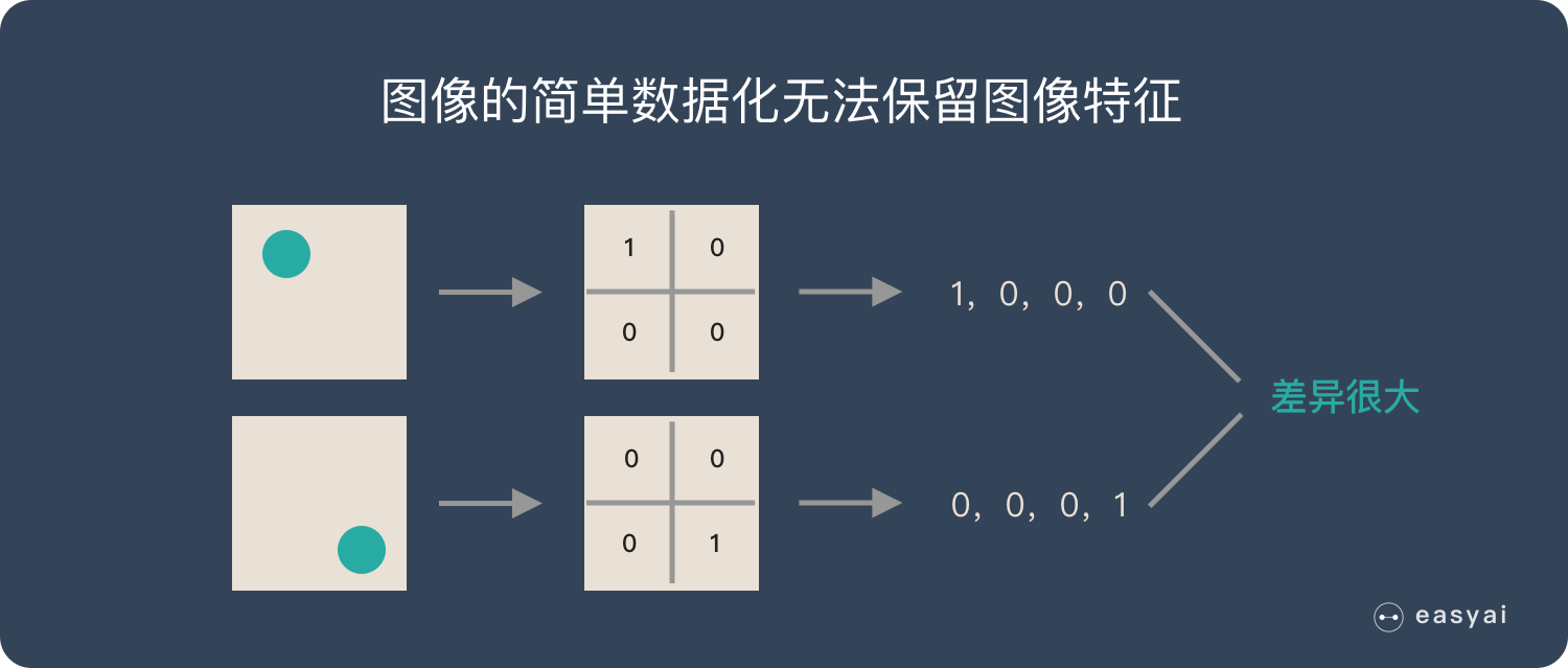
If a circle is 1 and no circle is 0, different positions of the circle will produce completely different data expressions. However, from the visual point of view, the content (essence) of the image has not changed, but the position has changed.
So when we move the object in the image, the parameters obtained in the traditional way will be very different! This does not meet the requirements of image processing.
CNN solves this problem. It retains the features of the image in a visual way. When the image is flipped, rotated or changed, it can also effectively recognize similar images.

Human visual principles

Many research results of deep learning are inseparable from the study of brain cognitive principle, especially the study of visual principle.
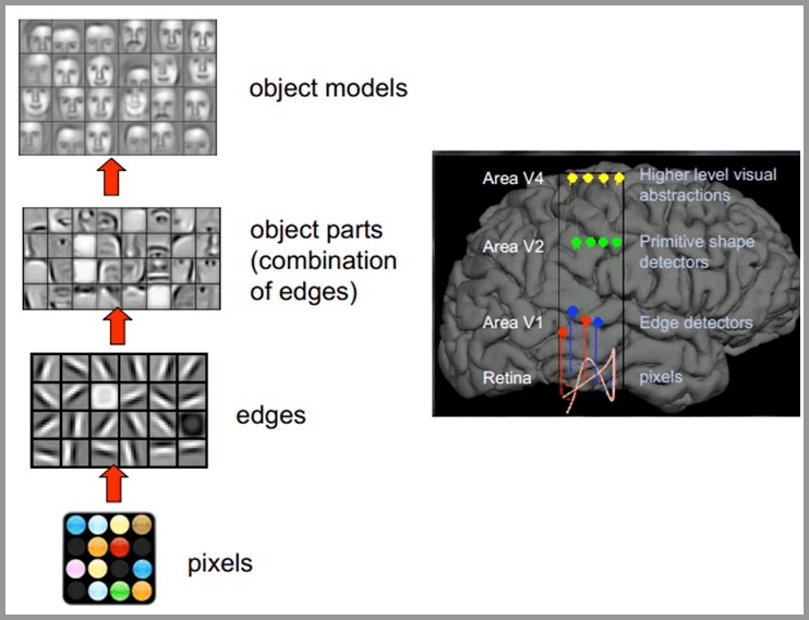
The principle of human vision is as follows: start with the intake of the original signal (the pupil intake Pixels), then do preliminary processing (some cells in the cerebral cortex find the edge and direction), then abstract (the brain determines that the shape of the object in front of you is round), and then further abstract (the brain further determines that the object is a balloon). The following is an example of human brain face recognition:

For different objects, human vision is also recognized by grading layer by layer:

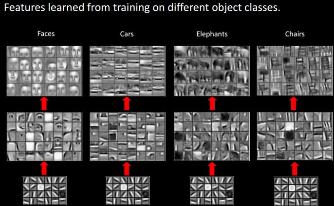
It can be clearly seen that the bottom features of different images are similar, that is, the higher the edges, the more they can extract some features of such objects (wheels, eyes, trunk, etc.), and to the top, the different high-level features will finally be combined into corresponding images, so that human beings can accurately distinguish different objects.
Therefore, we can imitate the characteristics of the human brain, construct a multi-layer neural network, recognize the primary image features at the lower level, and several lower level features form the upper level features. Finally, through the combination of multiple levels, we can finally make classification at the top level.

Basic principle of convolutional neural network CNN

A typical CNN consists of the following three layers
1. Convolution layer
2. Pool layer
3. Full connection layer
In short, the convolution layer is used to extract the local features of the image, the pooling layer is used for data dimensionality reduction, and the full connection layer is similar to the ordinary neural network to output the desired results.

Convolution local feature extraction

Convolution layer is one of the most important steps in CNN architecture. Basically, convolution is a linear and translation invariant operation, which consists of a combination of performing local weighting on the input signal.
There are several important concepts in alluvium:
1. local receptive fields
2. shared weights
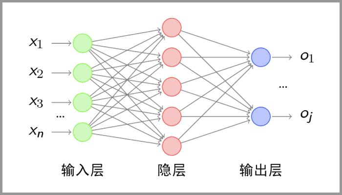
Suppose you enter a 5 × 5, we define 3 × A local receptive field of 3, that is, the neurons of the hidden layer and 5 of the input layer × Five neurons are connected.
It can be similarly seen that the neurons in the hidden layer have a fixed size sensory field to feel some characteristics of the upper layer. However, the perception field of vision is relatively small, and only some features of the upper layer can be seen. Other features of the upper layer can be obtained by translating the perception field of vision.
Set the moving step size as 1: scan from left to right, move 1 grid each time, move down one grid after scanning, and scan from left to right again. See the following for the specific process:

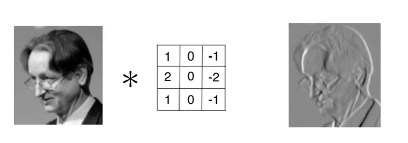
This process can be understood as that we use a filter (convolution kernel) to filter each small region of the image, so as to obtain the eigenvalues of these small regions. Different convolution kernels are used to extract some features (ex: shape) in the picture, just as the human brain infers what the picture is based on the shape. As shown in the figure below, the convolution kernel is used to extract the boundary of the picture:

It can be seen that the neurons of the convolution layer are only connected with some neuron nodes of the previous layer, and each connected line corresponds to a weight w. A receptive field has a convolution kernel. We call the weight w matrix in the receptive field as convolution kernel and the scanning interval between the receptive field and the input as stripe;

For all neurons in the lower layer, they detect the characteristics of neurons in the upper layer from different positions. We call the next layer neuron matrix generated by a sensory field scan with convolution kernel a feature map (feature map, the matrix on the right of the above figure is the feature map).
The neurons on the same feature map use the same convolution kernel, so these neurons share the weight, the weight in the convolution kernel and the accompanying offset.
In specific applications, there are often multiple convolution kernels. It can be considered that each convolution kernel represents an image mode. If the value of an image block convoluted with this convolution kernel is large, it is considered that this image block is very close to this convolution kernel. If we design six convolution kernels, we can understand that there are six underlying texture patterns on this image, that is, we can depict an image with six basic patterns. Here are examples of 25 different convolution kernels:
Conclusion: the convolution layer extracts the local features in the picture through the filtering of convolution kernel, which is similar to the feature extraction of human vision mentioned above.

Pooling layer (down sampling) - data dimensionality reduction to avoid over fitting

After convolution, the convolution layer usually makes a pooling layer after convolution. Commonly used pooling calculations include Max pooling, mean pooling, stochastic pooling, etc.
The pooling layer is simply down sampling, which can greatly reduce the dimension of data. The process is as follows

In the above figure, we can see that the original picture is 20 × 20, we down sample it, and the sampling window is 10 × 10. Finally, it will be down sampled into a 2 × 2 size feature map. The reason for this is that even after convolution, the image is still large (because the convolution kernel is relatively small), so in order to reduce the data dimension, down sampling is carried out.
Conclusion: compared with convolution layer, pooling layer can effectively reduce the data dimension. This can not only greatly reduce the amount of computation, but also effectively avoid over fitting.

Full connection layer - output results

This part is the last step. The data processed by the convolution layer and pooling layer is input to the full connection layer to get the final desired result, which plays the role of "Classifier" in the. After the dimensionality reduction of the convolution layer and pool layer, the full connection layer can "run". Otherwise, the amount of data is too large, the calculation cost is high and the efficiency is low.

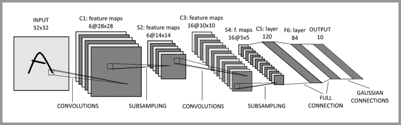
The typical CNN is not just the three-tier structure mentioned above, but a multi-tier structure. For example, the structure of LeNet-5 is shown in the figure below:

Implementation of convolutional neural network using pytorch – (MNIST actual combat)

import time
import torch.nn as nn
import matplotlib.pyplot as plt
from torchvision import transforms
from torch.utils.data import DataLoader
from torchvision.datasets import MNIST
from torch import optim

# Define batch, that is, the sample size of one training
train_batch_size = 128
test_batch_size = 128

# Define image data conversion operations
# transforms.Compose is used to integrate multiple steps together
# transforms.ToTensor can transform the gray range from 0-255 to 0-1, and the following transform Normalize() transforms 0-1 to (- 1,1)
# mnist is a gray-scale image and should be set as a single channel, so the mean and standard deviation of Normalize are [0.5]
transform = transforms.Compose([transforms.ToTensor(), transforms.Normalize([0.5], [0.5])])

# Download mnist data set. If it has been downloaded, download can be defined as False
data_train = MNIST('./data', train=True, transform=transform, target_transform=None, download=True)
data_test = MNIST('./data', train=True, transform=transform, target_transform=None, download=True)

train_loader = DataLoader(data_train, batch_size=train_batch_size, shuffle=True)
test_loader = DataLoader(data_test, batch_size=test_batch_size, shuffle=True)

# Visualization data, this step can be ignored
examples = enumerate(test_loader)
batch_idx, (example_data, example_targets) = next(examples)
plt.figure(figsize=(9, 9))
for i in range(9):
    plt.subplot(3, 3, i + 1)
    plt.title("Ground Truth:{}".format(example_targets[i]))
    plt.imshow(example_data[i][0], cmap='gray', interpolation='none')
    plt.xticks([])
    plt.yticks([])
plt.show()


# Build model
class CNN_net(nn.Module):
    def __init__(self):
        super(CNN_net, self).__init__()
        # Convolution layer
        self.conv1 = nn.Sequential(
            nn.Conv2d(1, 16, kernel_size=(3, 3), stride=(1, 1), padding=1),
            nn.ReLU(inplace=True),
            nn.MaxPool2d(kernel_size=2, stride=2)
        )
        self.conv2 = nn.Sequential(
            nn.Conv2d(16, 32, kernel_size=(3, 3), stride=(1, 1), padding=1),
            nn.ReLU(inplace=True),
            nn.MaxPool2d(kernel_size=2, stride=2)
        )

        # Full connection layer
        self.dense = nn.Sequential(
            nn.Linear(7 * 7 * 32, 128),
            nn.ReLU(),
            nn.Dropout(p=0.5),  # Alleviate over fitting and regularize to some extent
            nn.Linear(128, 10)
        )

    def forward(self, x):
        x = self.conv1(x)
        x = self.conv2(x)
        x = x.view(x.size(0), -1)  # The flatten tensor is flattened to facilitate the reception of the whole connection layer
        return self.dense(x)


model = CNN_net()
print(model)

# Set training parameters
learn_rate = 1e-3
epoches = 10

# loss function 
criterian = nn.CrossEntropyLoss()

# SGD for optimization
opt = optim.SGD(model.parameters(), lr=learn_rate, momentum=0.95)

# train
# Start training by defining an array that stores the loss function and accuracy
train_losses = []
train_acces = []
# test
eval_losses = []
eval_acces = []

print("start training...")
# Record the start time of training
start_time = time.time()

for epoch in range(epoches):
    # Training set
    train_loss = 0
    train_acc = 0
    # Set the model to training mode
    model.train()
    for img, label in train_loader:
        out = model(img)  # Returns the probability of each category
        loss = criterian(out, label)  # Calculate loss
        opt.zero_grad()  # Model gradient parameter reset
        loss.backward()  # Back propagation calculation completion error
        opt.step()  # Update parameters
        train_loss += loss  # Cumulative error
        _, pred = out.max(1)  # Returns the number of maximum probability
        num_correct = (pred == label).sum().item()  # Record the correct number of labels
        acc = num_correct / img.shape[0]  # Calculation accuracy
        train_acc += acc
    # Average deposit
    train_losses.append(train_loss / len(train_loader))
    train_acces.append(train_acc / len(train_loader))
    # Test set
    eval_loss = 0
    eval_acc = 0
    # Set the model to test mode
    model.eval()

    for img, label in test_loader:
        out = model(img)
        loss = criterian(out, label)
        opt.zero_grad()
        loss.backward()
        opt.step()

        eval_loss += loss

        _, pred = out.max(1)
        num_correct = (pred == label).sum().item()
        acc = num_correct / img.shape[0]
        eval_acc += acc
    eval_losses.append(eval_loss / len(test_loader))
    eval_acces.append(eval_acc / len(test_loader))

    # Output effect
    print('epoch:{},Train Loss:{:.4f},Train Acc:{:.4f},'
          'Test Loss:{:.4f},Test Acc:{:.4f}'
          .format(epoch, train_loss / len(train_loader),
                  train_acc / len(train_loader),
                  eval_loss / len(test_loader),
                  eval_acc / len(test_loader)))
    # Output duration
    stop_time = time.time()
    print("time is:{:.4f}s".format(stop_time - start_time))
print("end training.")

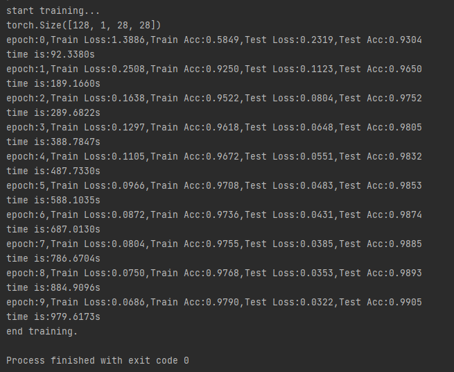
The operation results are as follows: