This is the study note of "hands-on deep learning" (PyTorch version) (dive into DL PyTorch). There are some codes that I expanded myself.

Other notes are in the column Deep learning Yes.

This is not simply copying the original content, but adding their own understanding. Almost all the codes in it have detailed comments!!!

6 linear neural network -- softmax regression

6.1 softmax regression

6.1.1 concept

In fact, we are often interested in classification: not "how much", but "which":

(1) Hard category: that is, which category it belongs to;

(2) Soft category: get the probability of belonging to each category.

A simple way to represent classified data: * * one hot encoding) * * is a vector with as many components as categories.

• softmax regression has multiple inputs and outputs (each category corresponds to one output), and requires as many affine functions as outputs. Each output corresponds to its own affine function.
• softmax regression is a single-layer neural network.
• The output layer of softmax regression is the full connection layer (each output depends on all inputs).
• The output of softmax regression is still determined by the affine transformation of input characteristics, which is a linear model.

6.1.2 softmax operation

(1) Operation formula

We must ensure that the output on any data is nonnegative (exponentiation of each non normalized prediction) and the sum is 1 (the result of each exponentiation divided by their sum):
o = x W + b \boldsymbol{o}=\boldsymbol{x} \boldsymbol{W}+\boldsymbol{b} o=xW+b

y ^ = softmax ⁡ ( o )   among   y ^ j = exp ⁡ ( o j ) ∑ k exp ⁡ ( o k ) \Hat {\ mathbf {y} = \ operatorname {softmax} (\ mathbf {o}) \ Quad \ text {where} \ quad \hat{y}_{j}=\frac{\exp \left(o_{j}\right)}{\sum_{k} \exp \left(o_{k}\right)} y^​=softmax(o)   among   y^​j​=∑k​exp(ok​)exp(oj​)​

(2) Cross entropy loss

• Cross entropy is often used to measure the difference between two probabilities H ( p , q ) = ∑ i − p i log ⁡ ( q i ) H(\mathbf{p}, \mathbf{q})=\sum_{i}-p_{i} \log \left(q_{i}\right) H(p,q)=∑i​−pi​log(qi​)
• Treat it as a loss
  l ( y , y ^ ) = − ∑ j = 1 q y j log ⁡ y ^ j = − log ⁡ y ^ y l(\mathbf{y}, \hat{\mathbf{y}})=-\sum_{j=1}^{q} y_{j} \log \hat{y}_{j}=-\log \hat{y}_{y} l(y,y^​)=−j=1∑q​yj​logy^​j​=−logy^​y​
  y i y_i Only one of yi equals 1, that is i = y i=y When i=y, so there's only one left y ^ y \hat{y}_{y} Y ^ y, synthesize the above formula:
  l ( y , y ^ ) = − ∑ j = 1 q y j log ⁡ exp ⁡ ( o j ) ∑ k = 1 q exp ⁡ ( o k ) = ∑ j = 1 q y j log ⁡ ∑ k = 1 q exp ⁡ ( o k ) − ∑ j = 1 q y j o j = log ⁡ ∑ k = 1 q exp ⁡ ( o k ) − ∑ j = 1 q y j o j \begin{aligned} l(\mathbf{y}, \hat{\mathbf{y}}) &=-\sum_{j=1}^{q} y_{j} \log \frac{\exp \left(o_{j}\right)}{\sum_{k=1}^{q} \exp \left(o_{k}\right)} \\ &=\sum_{j=1}^{q} y_{j} \log \sum_{k=1}^{q} \exp \left(o_{k}\right)-\sum_{j=1}^{q} y_{j} o_{j} \\ &=\log \sum_{k=1}^{q} \exp \left(o_{k}\right)-\sum_{j=1}^{q} y_{j} o_{j} \end{aligned} l(y,y^​)​=−j=1∑q​yj​log∑k=1q​exp(ok​)exp(oj​)​=j=1∑q​yj​logk=1∑q​exp(ok​)−j=1∑q​yj​oj​=logk=1∑q​exp(ok​)−j=1∑q​yj​oj​​
• Its gradient is the difference between real probability and prediction probability
  ∂ o j l ( y , y ^ ) = exp ⁡ ( o j ) ∑ k = 1 q exp ⁡ ( o k ) − y j = softmax ⁡ ( o ) j − y j \partial_{o_{j}} l(\mathbf{y}, \hat{\mathbf{y}})=\frac{\exp \left(o_{j}\right)}{\sum_{k=1}^{q} \exp \left(o_{k}\right)}-y_{j}=\operatorname{softmax}(\mathbf{o})_{j}-y_{j} ∂oj​​l(y,y^​)=∑k=1q​exp(ok​)exp(oj​)​−yj​=softmax(o)j​−yj​

Extension: several common loss functions

L2 Loss: l ( y , y ′ ) = 1 2 ( y − y ′ ) 2 l(y,y') = \frac{1}{2} (y-y')^2 l(y,y′)=21​(y−y′)2
L1 Loss: l ( y , y ′ ) = ∣ y − y ′ ∣ l(y,y') = |y-y'| l(y,y′)=∣y−y′∣
Huber's Robust Loss:
l ( y , y ′ ) = { ∣ y − y ′ ∣ − 1 2  if  ∣ y − y ′ ∣ > 1 1 2 ( y − y ′ ) 2  otherwise  l\left(y, y^{\prime}\right)= \begin{cases}\left|y-y^{\prime}\right|-\frac{1}{2} & \text { if }\left|y-y^{\prime}\right|>1 \\ \frac{1}{2}\left(y-y^{\prime}\right)^{2} & \text { otherwise }\end{cases} l(y,y′)={∣y−y′∣−21​21​(y−y′)2​ if ∣y−y′∣>1 otherwise ​
When the predicted value differs greatly from the actual value, it is the absolute value error; If the difference is small, it is the mean square error.

6.2 image classification dataset (fashion MNIST)

The most commonly used image classification dataset is the handwritten numeral recognition dataset MNIST. However, the classification accuracy of most models on MNIST exceeds 95%. In order to more intuitively observe the differences between algorithms, we will use a data set fashion MNIST with more complex image content (this data set is also relatively small, only tens of M, which can be endured by computers without GPU).

We first introduce a multi class image classification dataset to facilitate us to observe the differences in model accuracy and computational efficiency between comparison algorithms.

In this section, we will use the torchvision package, which serves the PyTorch deep learning framework and is mainly used to build computer vision models. Torchvision is mainly composed of the following parts:

1. torchvision.datasets: some functions for loading data and common data set interfaces;
2. torchvision.models: contains common model structures (including pre training models), such as AlexNet, VGG, ResNet, etc;
3. torchvision.transforms: commonly used image transformations, such as cropping, rotation, etc;
4. torchvision.utils: some other useful methods.

First import the required package or module.

%matplotlib inline
import torch
import torchvision
from torch.utils import data
from torchvision import transforms
from d2l import torch as d2l

d2l.use_svg_display()  #Use svg to display pictures with higher definition

6.2.1 reading data sets

Download and read the fashion MNIST dataset into memory through the built-in functions in the framework.

In the following code:

• transforms.ToTensor() converts a PIL picture with size (H x W x C) and data in [0, 255] or a NumPy array with data type np.uint8 to a Tensor with size (C x H x W) and data type torch.float32 and data in [0.0, 1.0].
• mnist_train and mnist_test is a subclass of torch.utils.data.Dataset, so we can use len() to get the size of the dataset and subscript to get a specific sample.
• Take out FashionMNIST from torchvision.datasets and download it to root.
• train=True indicates that the training data set is downloaded; train=False indicates that the test set is downloaded.
• transform=trans means that the data set of the corresponding PyTorch is taken out, not a pile of pictures.
• download=True means downloading from the Internet by default (you can also download it in advance and put it in data, so you don't need this command).

The output results (60000, 10000) represent mnist_train needs about 60000 pictures, mnist_test needs about 10000 images (the number of images in each category in the training set and test set is 6000 and 1000 respectively. Because there are 10 categories, the number of samples in the training set and test set is 60000 and 10000 respectively).

trans = transforms.ToTensor()  #The simplest preprocessing to convert an image into Tensor is to return a PIL image without conversion
mnist_train = torchvision.datasets.FashionMNIST(
    root="C:/Users/xinyu/Desktop/myjupyter/data", train=True, transform=trans, download=True)  #Training data set
mnist_test = torchvision.datasets.FashionMNIST(
    root="C:/Users/xinyu/Desktop/myjupyter/data", train=False, transform=trans, download=True)  
#The test data set is only used to evaluate the performance of the model, not to train the model

len(mnist_train), len(mnist_test)

(60000, 10000)

mnist_train[0][0].shape  

torch.Size([1, 28, 28])

The fashion MNIST dataset contains both graphics and labels. The first [0] represents the 0 example (picture data), the second [0] represents the picture, and if it is [1], it is the label.

The above results indicate:

• First, this picture is a torch's tensor
• Dimension is (C) × H × W) The first dimension is the number of channels, and the last two dimensions are the height and width of the image
• The data set is composed of gray-scale images, and the number of channels is 1
• The height and width of each input image are 28 pixels

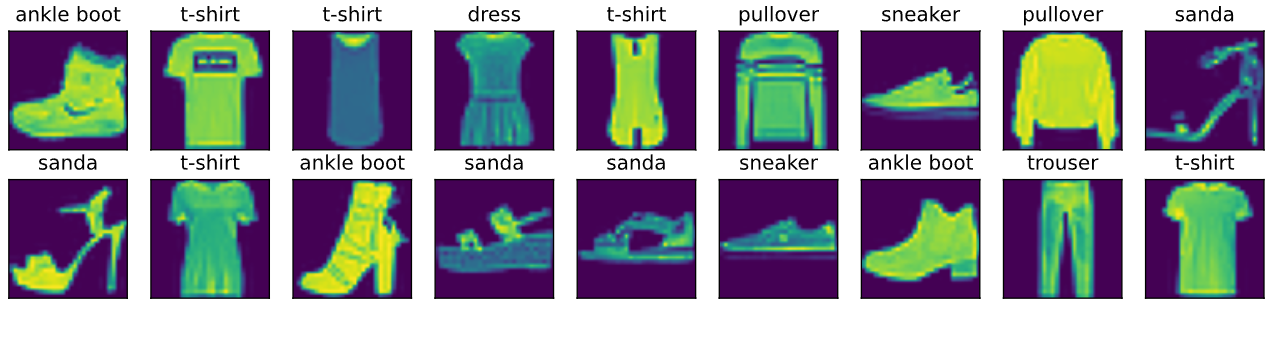
The 10 categories included in fashion MNIST are t-shirt, trouser, pullover, dress, coat, sandal, shirt, sneaker, bag and ankle boot. The following function is used to convert between a numeric label index and its text name.

def get_fashion_mnist_labels(labels):
    text_labels = ['t-shirt', 'trouser', 'pullover', 'dress', 'coat', 'sanda', 'shirt', 'sneaker', 'bag', 'ankle boot']
    return [text_labels[int(i)] for i in labels]

'''The following defines a function (visual sample) that can draw multiple images and corresponding labels in one line'''
def show_images(imgs, num_rows, num_cols, titles=None, scale=1.5):
    figsize = (num_cols * scale, num_rows * scale)
    _, axes = d2l.plt.subplots(num_rows, num_cols, figsize=figsize)  #Here_ Indicates that we ignore (do not use) variables
    axes = axes.flatten()
    for i, (ax, img) in enumerate(zip(axes, imgs)):
        if torch.is_tensor(img):  #Picture tensor
            ax.imshow(img.numpy())
        else:  #PIL picture
            ax.imshow(img)
        ax.axes.get_xaxis().set_visible(False)
        ax.axes.get_yaxis().set_visible(False)
        if titles:
            ax.set_title(titles[i])
    return axes

X, y = next(iter(data.DataLoader(mnist_train, batch_size=18)))  #next means to get the first small batch; Use iter to construct an iterate
show_images(X.reshape(18, 28, 28), 2, 9, titles=get_fashion_mnist_labels(y))  #18 samples, arranged in 2 rows and 9 columns, with a width and height of 28 (the width and height cannot be changed without authorization here)

array([<AxesSubplot:title={'center':'ankle boot'}>,
       <AxesSubplot:title={'center':'t-shirt'}>,
       <AxesSubplot:title={'center':'t-shirt'}>,
       <AxesSubplot:title={'center':'dress'}>,
       <AxesSubplot:title={'center':'t-shirt'}>,
       <AxesSubplot:title={'center':'pullover'}>,
       <AxesSubplot:title={'center':'sneaker'}>,
       <AxesSubplot:title={'center':'pullover'}>,
       <AxesSubplot:title={'center':'sanda'}>,
       <AxesSubplot:title={'center':'sanda'}>,
       <AxesSubplot:title={'center':'t-shirt'}>,
       <AxesSubplot:title={'center':'ankle boot'}>,
       <AxesSubplot:title={'center':'sanda'}>,
       <AxesSubplot:title={'center':'sanda'}>,
       <AxesSubplot:title={'center':'sneaker'}>,
       <AxesSubplot:title={'center':'ankle boot'}>,
       <AxesSubplot:title={'center':'trouser'}>,
       <AxesSubplot:title={'center':'t-shirt'}>], dtype=object)

6.2.2 read small batch

Use the built-in data iterator to read a small batch of data with the size of batch_size.

We will train the model on the training data set and evaluate the performance of the trained model on the test data set. As mentioned earlier, mnist_train is a subclass of torch.utils.data.Dataset, so we can pass it into torch.utils.data.DataLoader to create a DataLoader instance that reads small batch data samples

In practice, data reading is often the performance bottleneck of training, especially when the model is simple or the performance of computing hardware is high. A convenient feature of PyTorch's DataLoader is to allow multiple processes to speed up data reading. Here we pass the parameter num_workers to set up four processes to read data.

batch_size = 256

num_workers = 4  #Four processes are used to read data. Generally speaking, the picture may be placed on the hard disk (now our is already in memory), and multiple processes are required to read the data.

train_iter = data.DataLoader(mnist_train, batch_size, shuffle=True, num_workers=get_dataloader_workers())

timer = d2l.Timer()
for X, y in train_iter:
    continue
f'{timer.stop():.2f} sec'

'3.19 sec'

6.2.3 integration of all components

Now let's define load_data_fashion_mnist function, which is used to obtain and read the fashion MNIST dataset. It returns the data iterators for the training set and the validation set. In addition, it accepts an optional parameter to resize the image to another shape.

def load_data_fashion_mnist(batch_size, resize=None):  #@save
    #resize indicates whether to change the width and height
    """download Fashion-MNIST The dataset and then load it into memory."""
    trans = [transforms.ToTensor()]
    if resize:
        trans.insert(0, transforms.Resize(resize))
    trans = transforms.Compose(trans)
    mnist_train = torchvision.datasets.FashionMNIST(
        root="C:/Users/xinyu/Desktop/myjupyter/data", train=True, transform=trans, download=True)
    mnist_test = torchvision.datasets.FashionMNIST(
        root="C:/Users/xinyu/Desktop/myjupyter/data", train=False, transform=trans, download=True)
    return (data.DataLoader(mnist_train, batch_size, shuffle=True,
                            num_workers=get_dataloader_workers()),
            data.DataLoader(mnist_test, batch_size, shuffle=False,
                            num_workers=get_dataloader_workers()))

'''We specify resize Parameters to test load_data_fashion_mnist Function's image resizing function'''
train_iter, test_iter = load_data_fashion_mnist(32, resize=64)
for X, y in train_iter:
    print(X.shape, X.dtype, y.shape, y.dtype)
    break

torch.Size([32, 1, 64, 64]) torch.float32 torch.Size([32]) torch.int64

6.3 implementation of softmax regression from scratch

6.3.1 acquiring and reading data

import torch
from IPython import display
from d2l import torch as d2l

batch_size = 256
train_iter, test_iter = d2l.load_data_fashion_mnist(batch_size)  #Each time 256 pictures are read randomly, it returns to the iterator of the training set and the test set

6.3.2 initialization model parameters

Stretch the image into a vector. Each sample input is an image with a height and width of 28 pixels, and the length of the input vector of the model is 28 pixels × 28 = 784: each element of the vector corresponds to each pixel in the image.

Since the image has 10 categories and the number of outputs of the single-layer neural network output layer is 10, the weight and deviation parameters of softmax regression are 784 respectively × 10 and 1 × 10 matrix.

num_inputs = 784  
num_outputs = 10

W = torch.normal(0, 0.01, size=(num_inputs, num_outputs), requires_grad=True)  
#The weight is initialized to a Gaussian random distribution with a mean value of 0 and a variance of 0.01. The shape is 784 × ten
b = torch.zeros(num_outputs, requires_grad=True)  #Offset, shape is 1 × ten

6.3.3 realize softmax operation

Operate on multidimensional Tensor by dimension: give a Tensor matrix X. We can only sum the elements of the same column (dim=0) or the same row (dim=1), and keep the two dimensions of row and column in the result (keepdim=True).

X = torch.tensor([[1, 2, 3], 
                  [4, 5, 6]])
X.sum(0, keepdim=True), X.sum(1, keepdim=True)
#This is a 2 × 3 matrix, where sum followed by 0 means that the 0th element in X is transformed into 1, that is, X is 1 × 3 matrix; Sum followed by 1 means that the first element in X is changed into 1, that is, X is 2 × 1 matrix

(tensor([[5, 7, 9]]),
 tensor([[ 6],
         [15]]))

Implement softmax
softmax ⁡ ( X ) i j = exp ⁡ ( X i j ) ∑ k exp ⁡ ( X i k ) \operatorname{softmax}(\mathbf{X})_{i j}=\frac{\exp \left(\mathbf{X}_{i j}\right)}{\sum_{k} \exp \left(\mathbf{X}_{i k}\right)} softmax(X)ij​=∑k​exp(Xik​)exp(Xij​)​

def softmax(X):
    X_exp = torch.exp(X)
    partition = X_exp.sum(1, keepdim=True)
    return X_exp / partition  #The broadcast mechanism is applied here

'''Verify it softmax function'''
X = torch.normal(0, 1, (2, 5))  #Create a 2 with a mean of 0 and a variance of 1 × 5 matrix
X_prob = softmax(X)
X_prob, X_prob.sum(1), X_prob.sum(1, keepdim=True)

(tensor([[0.0784, 0.4247, 0.3255, 0.0969, 0.0746],
         [0.1576, 0.1277, 0.2073, 0.1265, 0.3810]]),
 tensor([1.0000, 1.0000]),
 tensor([[1.0000],
         [1.0000]]))

6.3.4 implement softmax regression model

o = x W + b \boldsymbol{o}=\boldsymbol{x} \boldsymbol{W}+\boldsymbol{b} o=xW+b

y ^ = softmax ⁡ ( o ) \hat{\mathbf{y}}=\operatorname{softmax}(\mathbf{o}) y^​=softmax(o)

def net(X):
    return softmax(torch.matmul(X.reshape((-1, W.shape[0])), W) + b)  
#X is an n × d (batch size) × Enter the matrix of (quantity). The number of samples (i.e. batch_size) corresponding to - 1 above, W.shape[0] is 784

6.3.5 calculation of loss function

Get the prediction probability of the label:

y = torch.tensor([0, 2])  #Indicates the label category of 2 samples (sample serial numbers are 0 and 1): Class 0 and class 2
y_hat = torch.tensor([[0.1, 0.3, 0.6], [0.3, 0.2, 0.5]])  #The prediction probability of these two samples in three categories (categories 0, 1 and 2)
y_hat[[0, 1], y]  #Take out the prediction probability of the 0 and 1 samples. y[0]=0, so take out 0.1; y[1]=2, so take out 0.5

tensor([0.1000, 0.5000])

Realize the cross entropy loss function:
l ( y , y ^ ) = − log ⁡ y ^ y l(\mathbf{y}, \hat{\mathbf{y}})=-\log \hat{y}_{y} l(y,y^​)=−logy^​y​

def cross_entropy(y_hat, y):
    return -torch.log(y_hat[range(len(y_hat)), y])  #With y above_ Hat [[0, 1], y] similarly, take out the probability for the real label

cross_entropy(y_hat, y)

tensor([2.3026, 0.6931])

6.3.6 calculation of classification accuracy

Given a category of prediction probability distribution y_hat, we take the category with the largest prediction probability as the output category. If it is consistent with the real category y, the prediction is correct. Classification accuracy refers to the ratio of correct forecast quantity to total forecast quantity. In the following code:

• y_hat.argmax(dim=1) returns matrix y_hat is the index of the largest element in each row, and the returned result is the same as the variable Y shape.
• The equality condition judgment formula (y_hat.argmax(dim=1) == y) is a Tensor of type ByteTensor. We use float() to convert it to a floating-point Tensor with a value of 0 (equality is false) or 1 (equality is true).

def accuracy(y_hat, y):  #@save
    return (y_hat.argmax(dim=1) == y).float().mean().item()

print(accuracy(y_hat, y))  

0.5

Above, the 0 and 1 samples we predicted are class 2 and class 2 respectively. In fact, they are Class 0 and class 2, that is, the accuracy is 50%, so the result is 0.5.

Similarly, we can evaluate the model net in the data iterator data_ Accuracy on ITER.

def evaluate_accuracy(data_iter, net):  #@save
    acc_sum, n = 0.0, 0
    for X, y in data_iter:
        acc_sum += (net(X).argmax(dim=1) == y).float().sum().item()
        n += y.shape[0]
    return acc_sum / n

print(evaluate_accuracy(test_iter, net))

0.0338

6.3.7 training model

The implementation of training softmax regression is very similar to the implementation of linear regression in the implementation from scratch section of linear regression. We also use small batch random gradient descent to optimize the loss function of the model. When training the model, the number of iteration cycles is num_epochs and learning rate lr are adjustable hyperparameters. Changing their values may result in a more accurate classification model.

num_epochs, lr = 5, 0.1

def train_ch3(net, train_iter, test_iter, loss, num_epochs, batch_size,
              params=None, lr=None, optimizer=None):  #@save
    for epoch in range(num_epochs):
        train_l_sum, train_acc_sum, n = 0.0, 0.0, 0
        for X, y in train_iter:
            y_hat = net(X)
            l = loss(y_hat, y).sum()

            # Gradient clearing
            if optimizer is not None:
                optimizer.zero_grad()
            elif params is not None and params[0].grad is not None:
                for param in params:
                    param.grad.data.zero_()

            l.backward()
            if optimizer is None:
                d2l.sgd(params, lr, batch_size)
            else:
                optimizer.step()  # The section "concise implementation of softmax regression" will be used


            train_l_sum += l.item()
            train_acc_sum += (y_hat.argmax(dim=1) == y).sum().item()
            n += y.shape[0]
        test_acc = evaluate_accuracy(test_iter, net)
        print('epoch %d, loss %.4f, train acc %.3f, test acc %.3f'
              % (epoch + 1, train_l_sum / n, train_acc_sum / n, test_acc))

train_ch3(net, train_iter, test_iter, cross_entropy, num_epochs, batch_size, [W, b], lr)

epoch 1, loss 0.7865, train acc 0.749, test acc 0.788
epoch 2, loss 0.5697, train acc 0.814, test acc 0.812
epoch 3, loss 0.5261, train acc 0.826, test acc 0.820
epoch 4, loss 0.5019, train acc 0.832, test acc 0.825
epoch 5, loss 0.4847, train acc 0.837, test acc 0.828

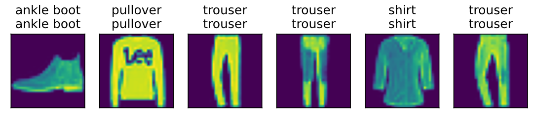
6.3.8 forecast

X, y = iter(test_iter).next()

trues = d2l.get_fashion_mnist_labels(y)
preds = d2l.get_fashion_mnist_labels(net(X).argmax(axis=1))
titles = [true +'\n' + pred for true, pred in zip(trues, preds)]

n = 6
d2l.show_images(X[0:n].reshape((n, 28, 28)), 1, n, titles=titles[0:n])

array([<AxesSubplot:title={'center':'ankle boot\nankle boot'}>,
       <AxesSubplot:title={'center':'pullover\npullover'}>,
       <AxesSubplot:title={'center':'trouser\ntrouser'}>,
       <AxesSubplot:title={'center':'trouser\ntrouser'}>,
       <AxesSubplot:title={'center':'shirt\nshirt'}>,
       <AxesSubplot:title={'center':'trouser\ntrouser'}>], dtype=object)

6.4 concise implementation of softmax regression

import torch
from torch import nn
from d2l import torch as d2l


batch_size = 256
train_iter, test_iter = d2l.load_data_fashion_mnist(batch_size)

# PyTorch does not implicitly adjust the shape of the input. So,
# We define a flatten layer in front of the linear layer to adjust the shape of the network input
# Flatten() converts the tensor of any dimension into two dimensions, retains the 0 dimension, and expands all the rest into a vector
# nn.Linear(784, 10) defines the linear layer. The input is 784 and the output is 10
net = nn.Sequential(nn.Flatten(), nn.Linear(784, 10))
 
def init_weights(m):  #Generate W
    if type(m) == nn.Linear:
        nn.init.normal_(m.weight, std=0.01)

net.apply(init_weights)

Sequential(
  (0): Flatten(start_dim=1, end_dim=-1)
  (1): Linear(in_features=784, out_features=10, bias=True)
)

loss = nn.CrossEntropyLoss()
trainer = torch.optim.SGD(net.parameters(), lr=0.1)

num_epochs = 10
d2l.train_ch3(net, train_iter, test_iter, loss, num_epochs, trainer)