1 perceptron

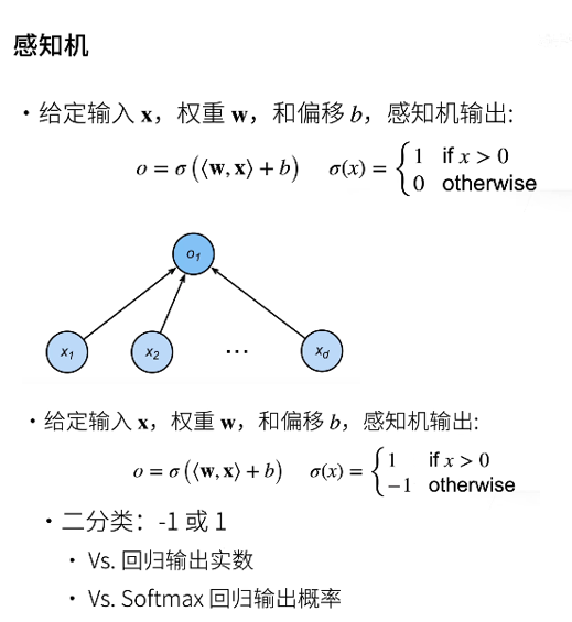
The output of the perceptron can be set to 0 or 1; Or - 1, 1.

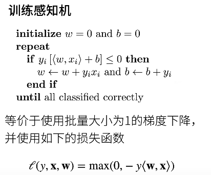
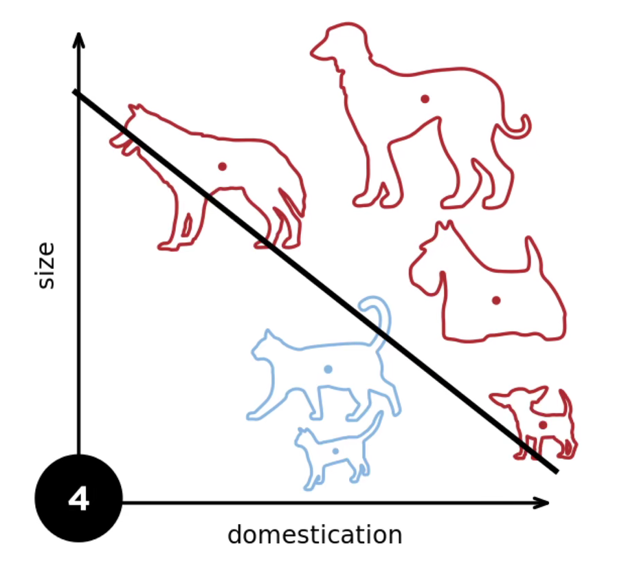
By continuously introducing data points, this line can effectively segment all kinds of training data.

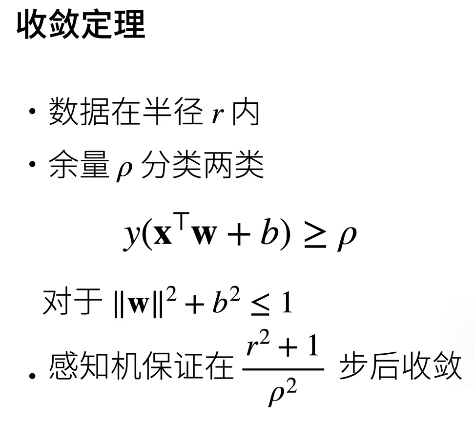
It is worth noting that the convergence theorem is a concept in mathematical statistics.

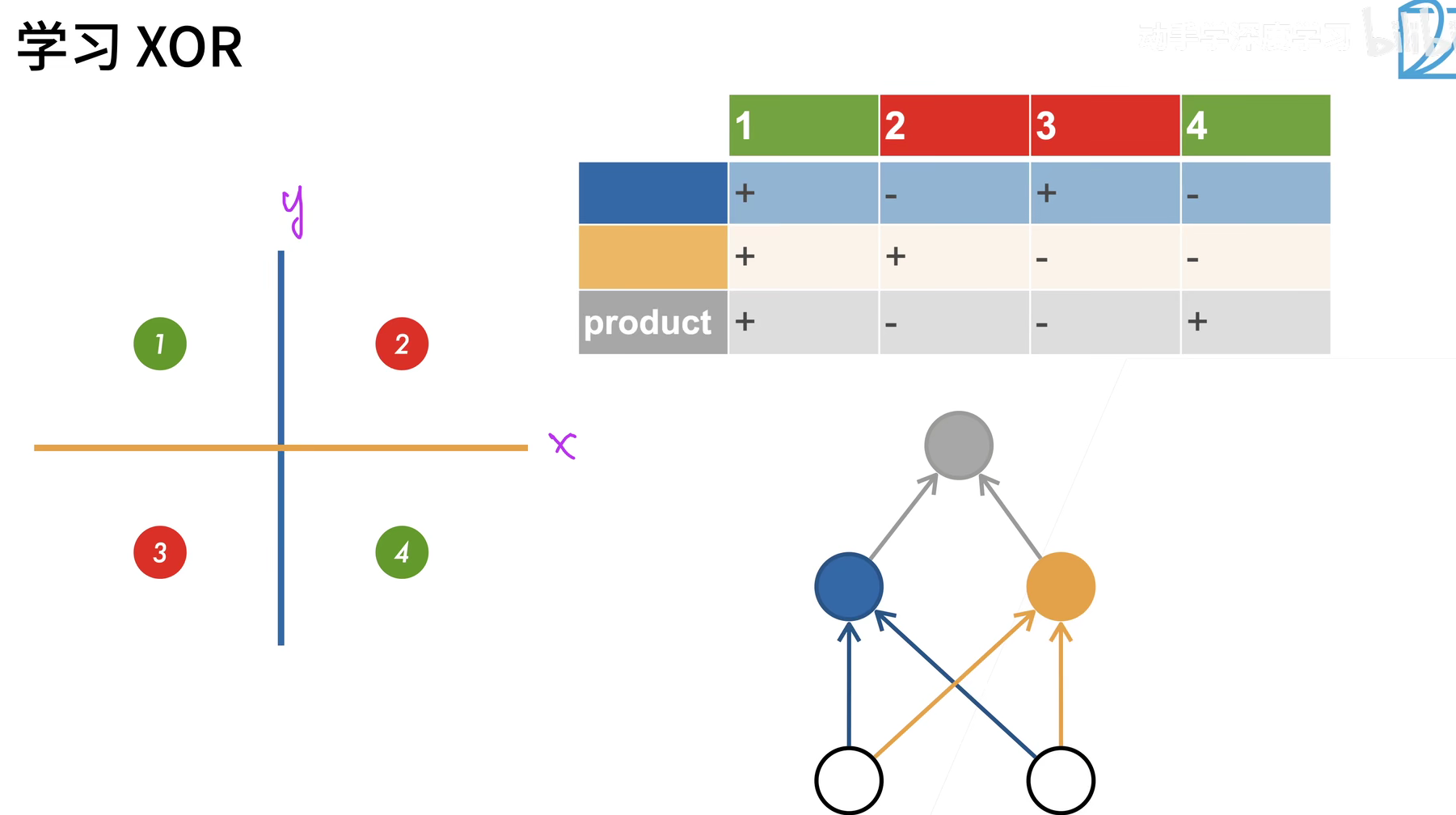
Points cannot be taken on the plane to separate such two data (red and green points).

2 multilayer perceptron

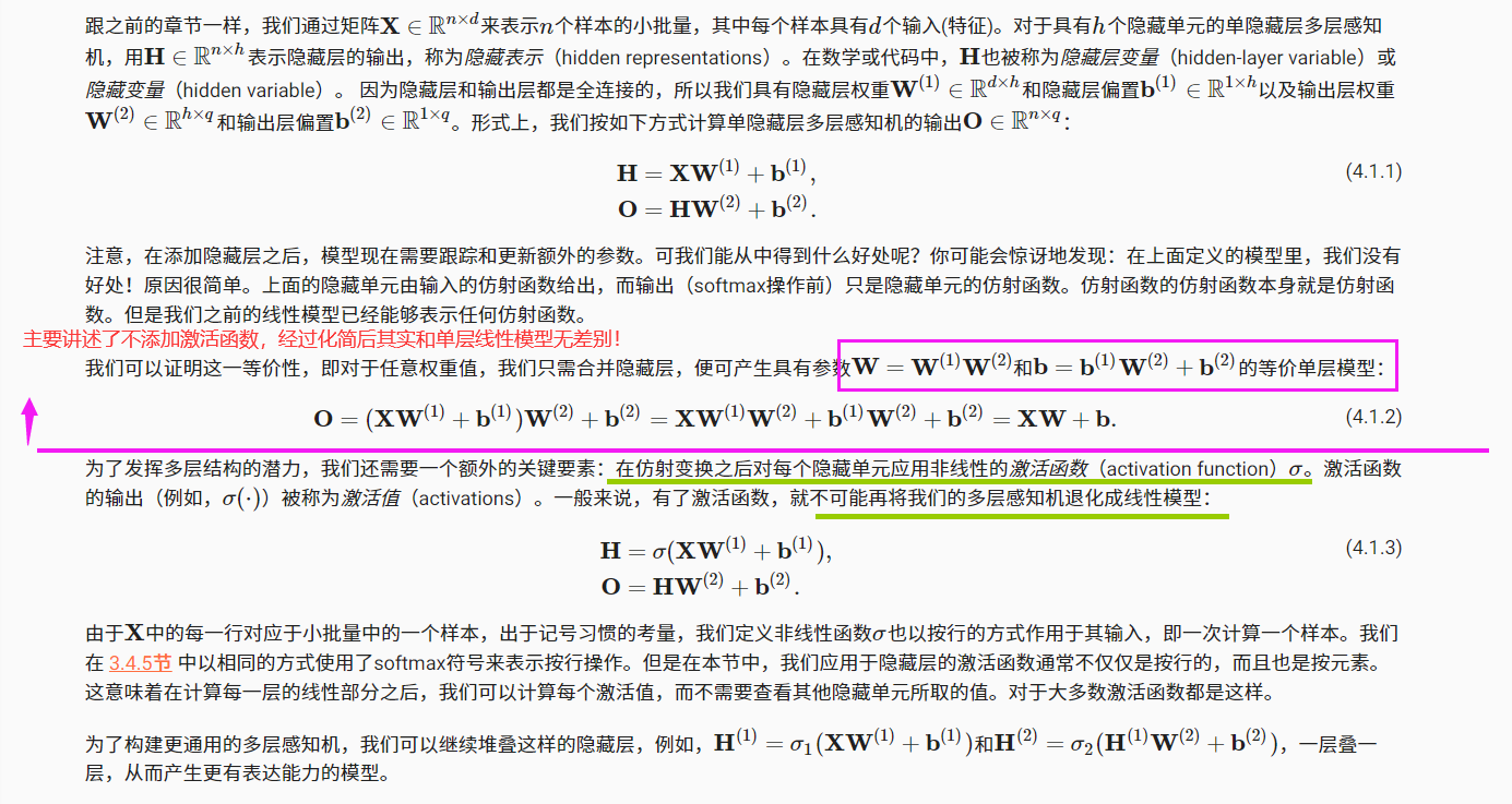
Recall the model structure of softmax regression. The model directly maps our input to the output through a single affine transformation, and then performs softmax operation.
If our tags are indeed related to our input data after affine transformation, this method is sufficient. However, linearity in affine transformation is a strong assumption.

But for many labels, it is not simply linear.

2.1 adding a hidden layer to the network

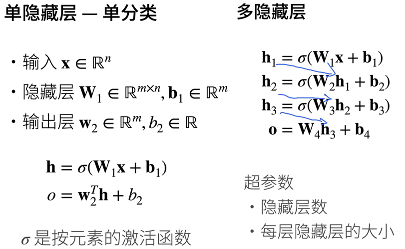
We can overcome the limitation of linear model by adding one or more hidden layers in the network, so that it can deal with more general functional relationship types.

The easiest way to do this is to stack many full connection layers together. Each layer is output to the upper layer until the final output is generated.

We can regard the first L − 1 layer as a full connection layer and the last layer as a linear predictor.

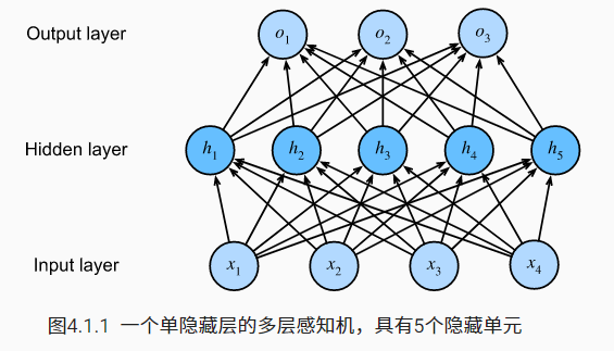
The multi-layer perceptron has 4 inputs and 3 outputs, and its hidden layer contains 5 hidden units. The input layer does not involve any calculation, so using this network to generate output only needs to realize the calculation of the hidden layer and the output layer; Therefore, the number of layers in this multilayer perceptron is 2.

2.2 variation of nonlinearity

2.3 common activation functions

The activation function determines whether a neuron should be activated by calculating a weighted sum and adding a bias. They are differentiable operations that convert input signals into outputs. Most activation functions are nonlinear

2.3.1 ReLU function

import torch
import matplotlib.pyplot as plt

x = torch.arange(-8.0, 8.0, 0.1, requires_grad=True)
y = torch.relu(x)
plt.figure(1)
plt.plot(x.detach(), y.detach())
plt.title('ReLU')

y.backward(torch.ones_like(x), retain_graph=True)
plt.figure(2)
plt.plot(x.detach(), x.grad)
plt.title('grad of relu')
plt.show()  # Show all pictures

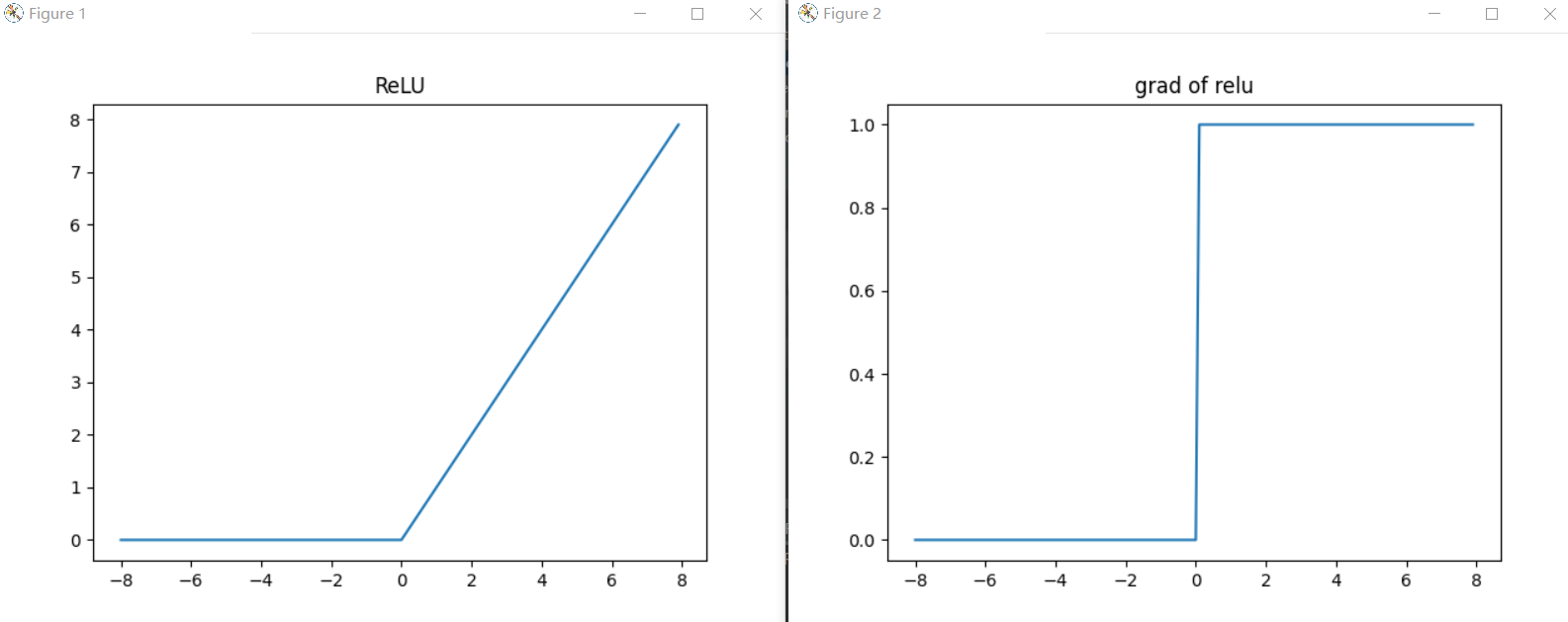
When the input is negative, the derivative of the ReLU function is 0, and when the input is positive, the derivative of the ReLU function is 1.

The reason for using ReLU is that its derivation performs particularly well: either let the parameter disappear or let the parameter pass.

2.3.2 sigmoid function

Just modify y = torch.sigmoid(x).

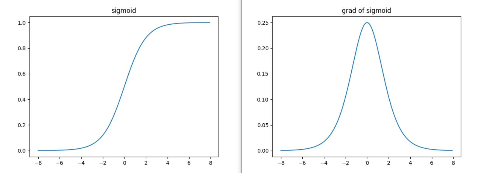
**Derivative of sigmoid function: * * when the input is 0, the derivative of sigmoid function reaches the maximum value of 0.25. The farther the input is from 0 in any direction, the closer the derivative is to 0.

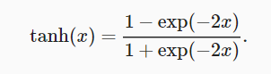
2.3.3 tanh function

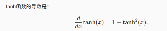
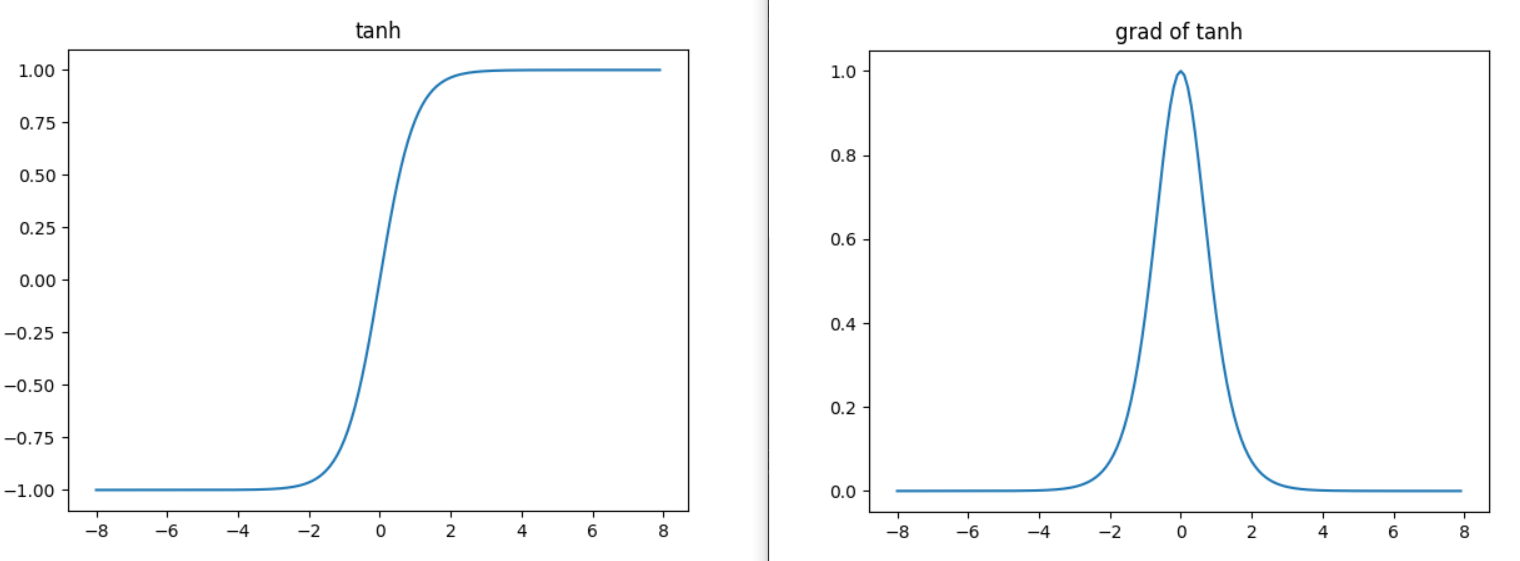
**Derivative of tanh function: * * when the input is close to 0, the derivative of tanh function is close to the maximum value of 1. Similar to what we see in the sigmoid function image, the farther the input is away from 0 in either direction, the closer the derivative is to 0.

3 implementation of multi-layer perceptron from scratch

import torch
from torch import nn
from d2l import torch as d2l
import matplotlib.pyplot as plt

3.1 initialize model parameters

Recall that each image in fashion MNIST consists of 28 × 28 = 784 gray pixel values. All images are divided into 10 categories. Ignoring the spatial structure between pixels, we can treat each image as a simple classification dataset with 784 input features and 10 classes

Generally, we choose several powers of 2 as the width of the layer. Because of the way memory is allocated and addressed in hardware, this can often be more computationally efficient.

num_inputs, num_outputs, num_hiddens = 784, 10, 256  # 256 is the number of hidden cells

W1 = nn.Parameter(torch.randn(
    num_inputs, num_hiddens, requires_grad=True) * 0.01)
b1 = nn.Parameter(torch.zeros(num_hiddens, requires_grad=True))
W2 = nn.Parameter(torch.randn(
    num_hiddens, num_outputs, requires_grad=True) * 0.01)
b2 = nn.Parameter(torch.zeros(num_outputs, requires_grad=True))

params = [W1, b1, W2, b2]

3.2 activation function

def relu(X):
    a = torch.zeros_like(X)
    return torch.max(X, a)

zeros_like function record:

a = torch.zeros_like(X) # constructs a matrix A whose dimension is consistent with matrix X
torch.max(X, a) # uses the maximum function to implement the ReLU activation function

3.3 model definition

def net(X):
    X = X.reshape((-1, num_inputs))
    H = relu(X@W1 + b1)  # Here "@" represents matrix multiplication
    return (H@W2 + b2)

3.4 loss function

Directly use the built-in functions in the advanced API to calculate softmax and cross entropy loss.

loss = nn.CrossEntropyLoss()

3.5 training

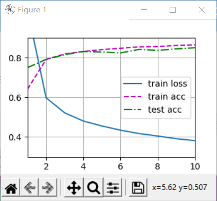
Fortunately, the training process of multi-layer perceptron is exactly the same as that of softmax regression. You can call the train of d2l package directly_ CH3 function.

num_epochs, lr = 10, 0.1
updater = torch.optim.SGD(params, lr=lr)
d2l.train_ch3(net, train_iter, test_iter, loss, num_epochs, updater)

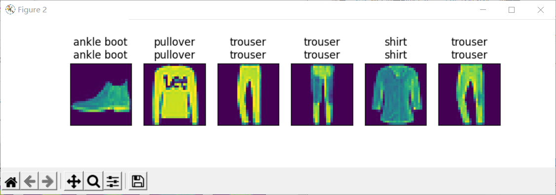
And make predictions:

d2l.predict_ch3(net, test_iter)

4 simple implementation of multi-layer perceptron

Compared with the concise implementation of softmax regression (: numref: sec_softmax_reason), the only difference is that we have added two full connection layers (we only added one full connection layer before).

net = nn.Sequential(nn.Flatten(),
                    nn.Linear(784, 256),  #From input layer to hidden layer 
                    nn.ReLU(),  # From hidden layer to output layer
                    nn.Linear(256, 10))

def init_weights(m):
    if type(m) == nn.Linear:
        nn.init.normal_(m.weight, std=0.01)

net.apply(init_weights);

batch_size, lr, num_epochs = 256, 0.1, 10
loss = nn.CrossEntropyLoss()
trainer = torch.optim.SGD(net.parameters(), lr=lr)

train_iter, test_iter = d2l.load_data_fashion_mnist(batch_size)
d2l.train_ch3(net, train_iter, test_iter, loss, num_epochs, trainer)

5 model selection, under fitting and over fitting

How can we make sure that the model really finds a generalized pattern instead of simply remembering the data?

5.1 training error and generalization error

training error refers to the error calculated by our model on the training data set. generalization error refers to the expectation of model error when we apply the model to an infinite number of data samples also extracted from the distribution of original samples.

We can never calculate the generalization error accurately. This is because the infinite number of data samples is a fictitious object. In practice, we can only estimate the generalization error by applying the model to an independent test set, which is composed of randomly selected data samples that do not appear in the training set.

5.2 model selection

In machine learning, we usually select the final model after evaluating several candidate models. This process is called model selection.
Sometimes, the models to be compared are completely different in nature (for example, decision tree and linear model). Sometimes, we need to compare the same kind of models under different hyperparametric settings. (for example, when training a multi-layer perceptron model, we may want to compare models with different numbers of hidden layers, different numbers of hidden units, and different combinations of activation functions.)

In theory, we use the training data to train the model, and use the test data to test the trained model. Moreover, the test data should not appear in the training data, and the test data should be discarded after being used once. But we rarely have enough data to use a new test set for each round of experiments.

The common way to solve this problem is to divide our data into three parts. In addition to training and testing data sets, we also add a validation data set, also known as validation set. But the reality is that the boundary between validation data and test data is worrisome.

K cross validation:

When training data is scarce, we may not even be able to provide enough data to form a suitable verification set. A popular solution to this problem is to use k-fold cross validation. Here, the original training data is divided into k non overlapping subsets. Then perform K times of model training and verification, train on the K − 1 subset each time, and verify on the remaining subset (there is no subset for training in this round). Finally, the training and verification errors are estimated by averaging the results of K experiments.

In depth learning, the training set is generally large, so the training cost of cross validation in depth learning is too high.

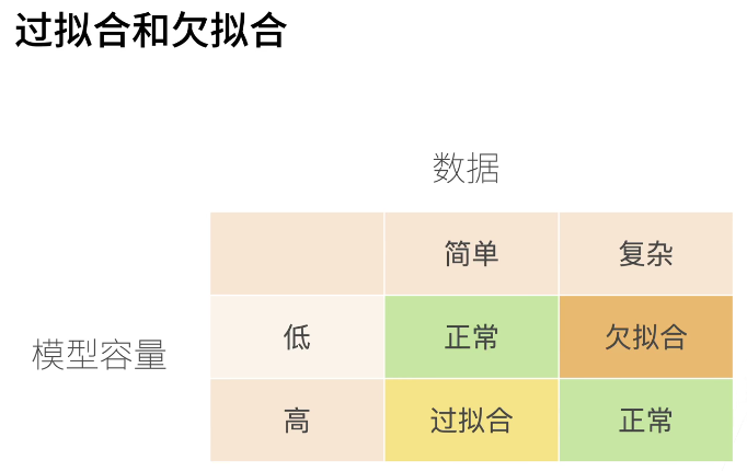
5.3 over fitting or under fitting

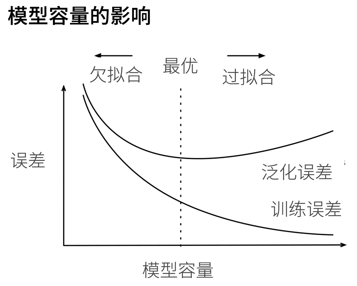
This picture is easy to understand. When the capacity of our model is low, the model can not fit the training set well, resulting in great training error and poor generalization ability of the model; When the capacity of the model is large, it is obvious that all the data of the test set can be fitted, and the training error is naturally very small. However, when dealing with a new data, the generalization error is very large due to over fitting.

Whether it is over fit or under fit may depend on the complexity of the model and the size of the available training data set.

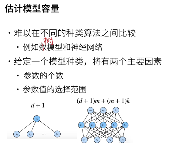
Model complexity

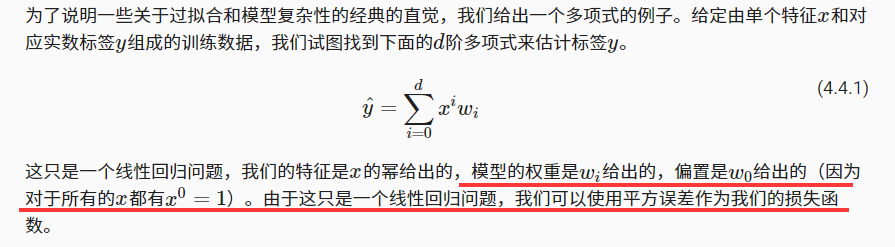
Higher order polynomial functions are much more complex than lower order polynomial functions. There are many parameters of higher-order polynomials and a wide range of model functions. Therefore, in the case of fixed training data set, the training error of high-order polynomial function should always be lower than that of low-order polynomial.

Dataset size

The fewer samples in the training data set, the more likely we are to encounter fitting. As the amount of training data increases, the generalization error usually decreases.

There is usually a relationship between model complexity and dataset size. Given more data, we may try to fit a more complex model.

5.4 polynomial regression

import math
import numpy as np
import torch
from torch import nn
from d2l import torch as d2l
import matplotlib.pyplot as plt

5.4.1 generating data sets

max_degree = 20
n_train, n_test = 100, 100
true_w = np.zeros(max_degree)  # [0. 0. 0. 0. 0. 0. 0. 0. 0. 0. 0. 0. 0. 0. 0. 0. 0. 0. 0. 0.]

features = np.random.normal(size=(n_train + n_test, 1))  # (200, 1)
np.random.shuffle(features)  # Scramble data

poly_features = np.power(features, np.arange(max_degree).reshape(1, -1))  # ((200, 1), (20, 1)) =(200, 20)
for i in range(max_degree):
    poly_features[:, 1] /= math.gamma(i + 1)
labels = np.dot(poly_features, true_w)
labels += np.random.normal(scale=0.1, size=labels.shape)

# NumPy ndarray to tensor
true_w, features, poly_features, labels = [torch.tensor(x, dtype=
    d2l.float32) for x in [true_w, features, poly_features, labels]]
    
print(features[:2], poly_features[:2, :], labels[:2])

Function notes:

power(x1, x2) to the power of x2 for each element in x1.
gamma(n) = (n-1)!;

5.4.2 training and testing the model

Implement a function to evaluate the loss of the model on a given data set.

def evaluate_loss(net, data_iter, loss):  # Import data and loss function
    """Evaluate the loss of the model on a given dataset."""
    metric = d2l.Accumulator(2)  # Sum of losses, number of samples
    for X, y in data_iter:
        out = net(X)
        y = y.reshape(out.shape)
        l = loss(out, y)
        metric.add(l.sum(), l.numel())
    return metric[0] / metric[1]

Now define the training function.

def train(train_features, test_features, train_labels, test_labels,
          num_epochs=400):
    loss = nn.MSELoss()
    input_shape = train_features.shape[-1]
    # No bias is set because we have implemented it in polynomial features
    net = nn.Sequential(nn.Linear(input_shape, 1, bias=False))
    batch_size = min(10, train_labels.shape[0])
    train_iter = d2l.load_array((train_features, train_labels.reshape(-1,1)),
                                batch_size)
    test_iter = d2l.load_array((test_features, test_labels.reshape(-1,1)),
                               batch_size, is_train=False)
    trainer = torch.optim.SGD(net.parameters(), lr=0.01)
    animator = d2l.Animator(xlabel='epoch', ylabel='loss', yscale='log',
                            xlim=[1, num_epochs], ylim=[1e-3, 1e2],
                            legend=['train', 'test'])
    for epoch in range(num_epochs):
        d2l.train_epoch_ch3(net, train_iter, loss, trainer)
        if epoch == 0 or (epoch + 1) % 20 == 0:
            animator.add(epoch + 1, (evaluate_loss(net, train_iter, loss),
                                     evaluate_loss(net, test_iter, loss)))
    print('weight:', net[0].weight.data.numpy())

# Select the first 4 dimensions from polynomial features, i.e. 1, x, x^2/2!, x^3/3!
train(poly_features[:n_train, :4], poly_features[n_train:, :4],
      labels[:n_train], labels[n_train:])
plt.show()

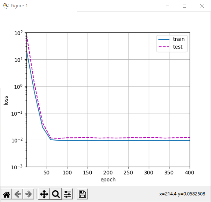
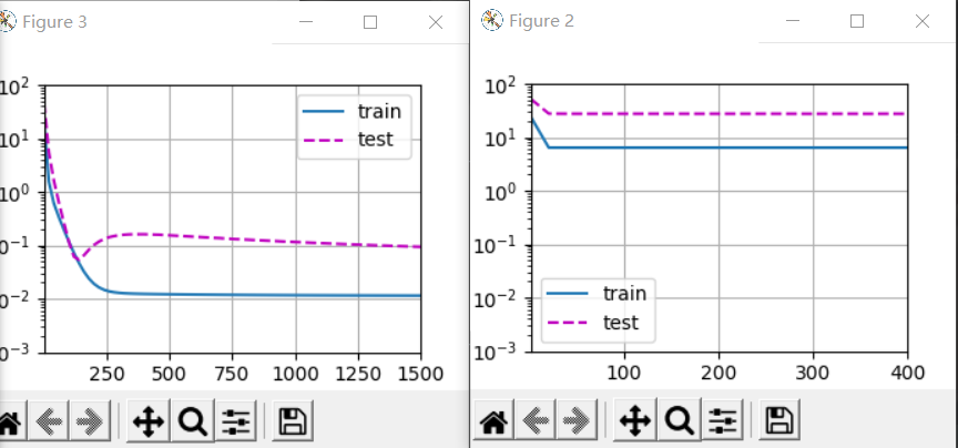
Linear function fitting (under fitting)

# Select the first 2 dimensions from polynomial features, i.e. 1, x
train(poly_features[:n_train, :2], poly_features[n_train:, :2],
      labels[:n_train], labels[n_train:])

High order polynomial function fitting (over fitting)

# Select all dimensions from polynomial features
train(poly_features[:n_train, :], poly_features[n_train:, :],
      labels[:n_train], labels[n_train:], num_epochs=1500)

6 weight decline

We have described the problem of over fitting, and now we can introduce some techniques of regularization model.

In the example of polynomial regression, we can limit the capacity of the model by adjusting the order of the fitting polynomial. In fact, limiting the number of features is a common technique to alleviate over fitting. However, simply discarding features may be too blunt for this work.

6.1 norm and weight decay

When training parametric machine learning models, * * weight attenuation (commonly known as L2 regularization) * * is one of the most widely used regularization techniques.

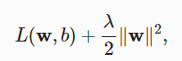
To ensure that the weight vector is relatively small, the most common method is to add its norm as a penalty term to the problem of minimizing loss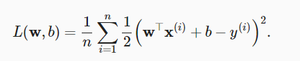

The original training objective minimizes the prediction loss on the training label and is adjusted to minimize the sum of prediction loss and penalty term.

In order to punish the size of the weight vector, we must add ‖ w ‖ 2 to the loss function in some way, but how should the model balance the loss of this new additional penalty? In fact, we use the regularization constant λ To describe this trade-off, this is a nonnegative hyperparameter.

L2 regularized linear model constitutes the classical ridge regression algorithm. L1 regularized linear regression is a similar basic model in statistics, which is usually called lasso regression.

One reason for using L2 norm is that it imposes huge penalties on large components of the weight vector.

Weight attenuation provides us with a continuous mechanism to adjust the complexity of the function. Smaller λ Values correspond to less constrained w and larger w λ Value has a greater constraint on w.

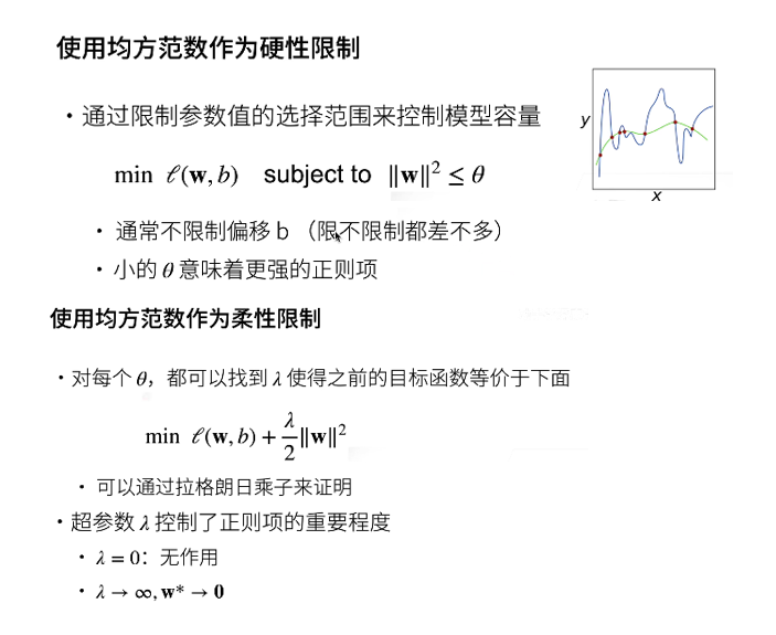
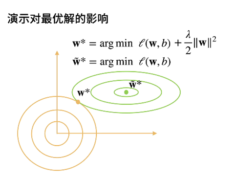
Lagrange multiplier method was originally used to solve the extreme value problem of multivariate function under constraints. For example, find the minimum value of F (x, y), but there is a constraint C(x,y) = 0. The general idea given by the multiplier method is to construct a new function g(x,y, λ) = f(x,y) + λ C(x,y), when gx = gy = 0 (partial derivative) is satisfied at the same time, the function takes the minimum value. The geometric meaning of this conclusion is that when f (x, y) is tangent to the contour line of C(x,y), the minimum value is taken.

Specifically to machine learning, C(x,y) = w^2- θ. So the yellow circle in the video represents different θ Constraints under. θ The smaller, the closer the final parameter is to the origin.

Summary:

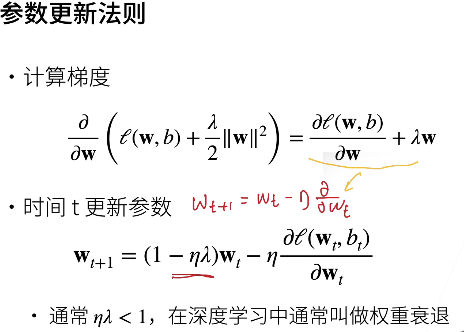
L2 regularization is to directly add a regularization term to the objective function, which directly modifies our optimization objective.

Weight attenuation is to directly cut a certain proportion of the parameter values in the network at the end of each step of training, and the formula of the optimization objective is unchanged.

You should know that there are many methods to avoid over fitting: early stopping, Data augmentation, Regularization, including L1, L2 (L2 regularization, also known as weight decay), dropout, not limited to weight decay.

6.2 realize from scratch

6.2.1 generating data

import torch
from torch import nn
from d2l import torch as d2l
import matplotlib.pyplot as plt

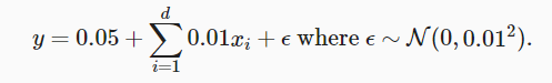
n_train, n_test, num_inputs, batch_size = 20, 100, 200, 5
true_w, true_b = torch.ones((num_inputs, 1)) * 0.01, 0.05
train_data = d2l.synthetic_data(true_w, true_b, n_train)
train_iter = d2l.load_array(train_data, batch_size)
test_data = d2l.synthetic_data(true_w, true_b, n_test)
test_iter = d2l.load_array(test_data, batch_size, is_train=False)

Function record:

synthetic_data(w, b, num_examples):
Generate y = Xw + b + noise.

6.2.2 initialization model parameters

def init_params():
    w = torch.normal(0, 1, size=(num_inputs, 1), requires_grad=True)
    b = torch.zeros(1, requires_grad=True)
    return [w, b]

6.2.3 define L2 norm penalty

def l2_penalty(w):
    return torch.sum(w.pow(2)) / 2

6.2.4 define training code implementation

def train(lambd):
    w, b = init_params()
    net, loss = lambda X: d2l.linreg(X, w, b), d2l.squared_loss
    num_epochs, lr = 100, 0.003
    animator = d2l.Animator(xlabel='epochs', ylabel='loss', yscale='log',
                            xlim=[5, num_epochs], legend=['train', 'test'])
    for epoch in range(num_epochs):
        for X, y in train_iter:
            with torch.enable_grad():
                # L2 norm penalty is added, and the broadcast mechanism makes l2_penalty(w) a vector with length of 'batch_size'.
                l = loss(net(X), y) + lambd * l2_penalty(w)  # Total loss
            l.sum().backward()
            d2l.sgd([w, b], lr, batch_size)
        if (epoch + 1) % 5 == 0:
            animator.add(epoch + 1, (d2l.evaluate_loss(net, train_iter, loss),
                                     d2l.evaluate_loss(net, test_iter, loss)))
    print('w of L2 The norm is:', torch.norm(w).item())

train(lambd=0)
plt.figure(1)
plt.plot

train(lambd=3)
plt.figure(2)
plt.plot
plt.show()

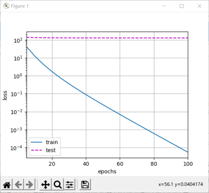
Note that here the training error increases, but the test error decreases. This is exactly what we expect from regularization. The over fitting is improved.

6.3 concise implementation

def train_concise(wd):
    net = nn.Sequential(nn.Linear(num_inputs, 1))
    for param in net.parameters():
        param.data.normal_()
    loss = nn.MSELoss()
    num_epochs, lr = 100, 0.003
    # The offset parameter has no attenuation.
    trainer = torch.optim.SGD([
        {"params": net[0].weight, 'weight_decay': wd},
        {"params": net[0].bias}], lr=lr)
    animator = d2l.Animator(xlabel='epochs', ylabel='loss', yscale='log',
                            xlim=[5, num_epochs], legend=['train', 'test'])
    for epoch in range(num_epochs):
        for X, y in train_iter:
            with torch.enable_grad():
                trainer.zero_grad()
                l = loss(net(X), y)
            l.backward()
            trainer.step()
        if (epoch + 1) % 5 == 0:
            animator.add(epoch + 1, (d2l.evaluate_loss(net, train_iter, loss),
                                     d2l.evaluate_loss(net, test_iter, loss)))
    print('w of L2 Norm:', net[0].weight.norm().item())


train_concise(wd=0)
plt.figure(1)
plt.plot

train_concise(wd=3)
plt.figure(2)
plt.plot
plt.show()

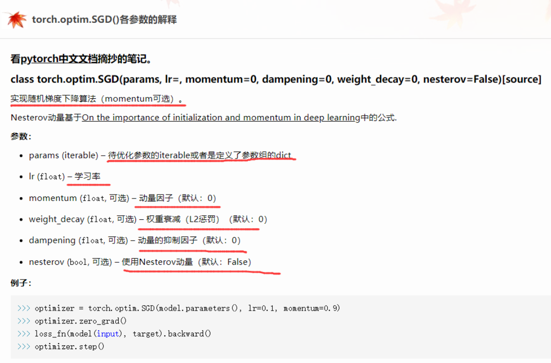
Function record:

torch.optim.SGD([{"params": net[0].weight, 'weight_decay': wd},
				{"params": net[0].bias}], lr=lr)

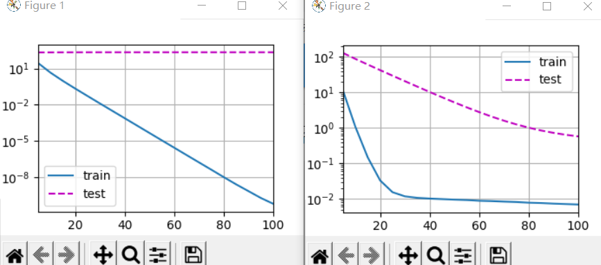
These graphs look the same as when we implemented weight attenuation from scratch. However, they run faster and easier to implement, and this benefit will become more obvious for more complex problems.