In the last chapter, we introduced the basic principle of convolutional neural network. In this chapter, we will take you to understand the structure of modern convolutional neural network. Many studies of modern convolutional neural network are based on this chapter.

Although the concept of deep neural networks is very simple - stacking neural networks together. However, due to different network structures and super parameter selection, the performance of these neural networks will change greatly.

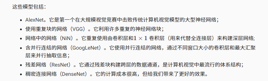
1 Deep convolution neural network AlexNet

1.1 model design

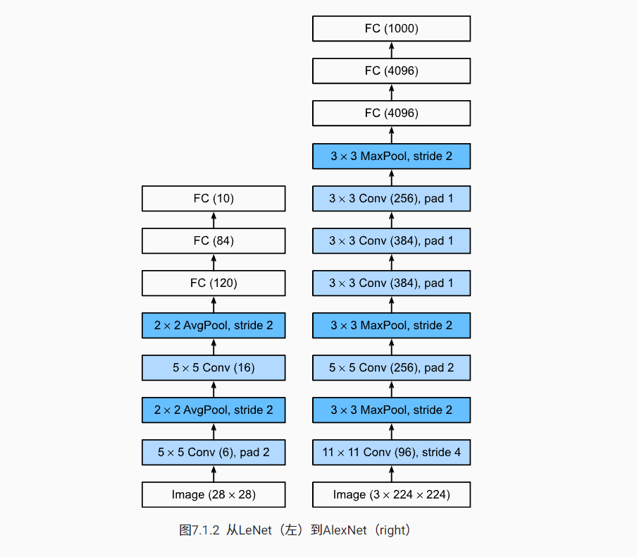
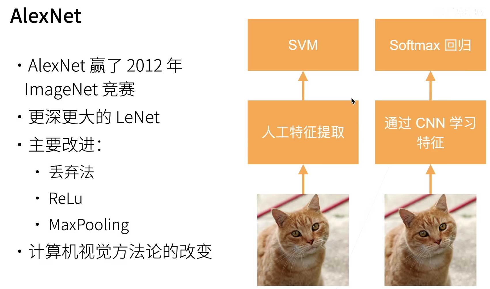
The design concepts of AlexNet and LeNet are very similar, but there are also significant differences. First, AlexNet is much deeper than the relatively small LeNet5. AlexNet consists of eight layers: five convolution layers, two fully connected hidden layers and one fully connected output layer. Second, AlexNet uses ReLU instead of sigmoid as its activation function.

1.2 capacity control and pretreatment

AlexNet controls the model complexity of the full connection layer through dropout, while LeNet only uses weight attenuation. In order to further expand the data, AlexNet adds a large amount of image enhancement data during training, such as flipping, clipping and color change. This makes the model more robust and the larger sample size effectively reduces over fitting.

import torch
from torch import nn
from d2l import torch as d2l

net = nn.Sequential(
    # Here, we use a larger window of 11 * 11 to capture objects.
    # At the same time, the stride is 4 to reduce the height and width of the output.
    # In addition, the number of output channels is much larger than LeNet
    nn.Conv2d(1, 96, kernel_size=11, stride=4, padding=1), nn.ReLU(),
    nn.MaxPool2d(kernel_size=3, stride=2),
    # Reduce the convolution window, fill it with 2 to make the height and width of input and output consistent, and increase the number of output channels
    nn.Conv2d(96, 256, kernel_size=5, padding=2), nn.ReLU(),
    nn.MaxPool2d(kernel_size=3, stride=2),
    # Three consecutive convolution layers and smaller convolution windows are used.
    # In addition to the last convolution layer, the number of output channels increases further.
    # After the first two convolution layers, the convergence layer is not used to reduce the height and width of the input
    nn.Conv2d(256, 384, kernel_size=3, padding=1), nn.ReLU(),
    nn.Conv2d(384, 384, kernel_size=3, padding=1), nn.ReLU(),
    nn.Conv2d(384, 256, kernel_size=3, padding=1), nn.ReLU(),
    nn.MaxPool2d(kernel_size=3, stride=2),
    nn.Flatten(),
    # Here, the number of outputs in the full connection layer is several times that in LeNet. Use the dropout layer to mitigate overfitting
    nn.Linear(6400, 4096), nn.ReLU(),
    nn.Dropout(p=0.5),
    nn.Linear(4096, 4096), nn.ReLU(),
    nn.Dropout(p=0.5),
    # Finally, the output layer. Since fashion MNIST is used here, the number of categories is 10 instead of 1000 in the paper
    nn.Linear(4096, 10))

We construct a single channel data with a height and width of 224 to observe the shape of the output of each layer.

X = torch.randn(1, 1, 224, 224)
for layer in net:
    X=layer(X)
    print(layer.__class__.__name__, 'Output shape:\t', X.shape)
################
Conv2d Output shape:	 torch.Size([1, 96, 54, 54])
ReLU Output shape:	 torch.Size([1, 96, 54, 54])
MaxPool2d Output shape:	 torch.Size([1, 96, 26, 26])
Conv2d Output shape:	 torch.Size([1, 256, 26, 26])
ReLU Output shape:	 torch.Size([1, 256, 26, 26])
MaxPool2d Output shape:	 torch.Size([1, 256, 12, 12])
Conv2d Output shape:	 torch.Size([1, 384, 12, 12])
ReLU Output shape:	 torch.Size([1, 384, 12, 12])
Conv2d Output shape:	 torch.Size([1, 384, 12, 12])
ReLU Output shape:	 torch.Size([1, 384, 12, 12])
Conv2d Output shape:	 torch.Size([1, 256, 12, 12])
ReLU Output shape:	 torch.Size([1, 256, 12, 12])
MaxPool2d Output shape:	 torch.Size([1, 256, 5, 5])
Flatten Output shape:	 torch.Size([1, 6400])
Linear Output shape:	 torch.Size([1, 4096])
ReLU Output shape:	 torch.Size([1, 4096])
Dropout Output shape:	 torch.Size([1, 4096])
Linear Output shape:	 torch.Size([1, 4096])
ReLU Output shape:	 torch.Size([1, 4096])
Linear Output shape:	 torch.Size([1, 10])

1.3 reading data sets

Although Alex net is trained on ImageNet in this article, we use the fashion MNIST dataset here. Because even on modern GPU s, it may take hours or days to train the ImageNet model and make it converge at the same time. One problem with the direct application of AlexNet to fashion MNIST is the resolution of fashion MNIST image (28) × 28 pixels) below the ImageNet image. To solve this problem, we increase them to 224 × 224 (generally speaking, this is not a wise practice, but we do it here to effectively use the AlexNet structure). We use D2L. Load_ data_ fashion_ The resize parameter in the MNIST function performs this adjustment.

batch_size = 128
train_iter, test_iter = d2l.load_data_fashion_mnist(batch_size, resize=224)

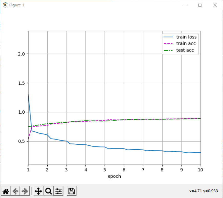
1.4 training AlexNet

lr, num_epochs = 0.01, 10
d2l.train_ch6(net, train_iter, test_iter, num_epochs, lr, d2l.try_gpu())
plt.show()

1.5 summary

• The structure of AlexNet is similar to LeNet, but more convolution layers and more parameters are used to fit large-scale ImageNet data sets.
• Today, AlexNet has been surpassed by a more effective structure, but it is a key step from shallow network to deep network.
• Although AlexNet has only a few more lines of code than LeNet, it took many years for academia to accept the concept of deep learning and apply its excellent experimental results. This is also due to the lack of effective calculation tools.
• Dropout, ReLU and preprocessing are other key steps to improve the performance of computer vision tasks.

2 network VGG using block

Although AlexNet has proved the effectiveness of deep neural network, it does not provide a general template to guide subsequent researchers to design new networks. In the following, we will introduce some heuristic concepts commonly used in the design of deep neural networks.

2.1. VGG block

The basic component of classical convolutional neural network is the following sequence:
① Convolution layer with filling to maintain resolution;
② Nonlinear activation function, such as ReLU;
③ Convergence layer, such as maximum convergence layer.

A VGG block is similar, which is composed of a series of convolution layers, followed by the maximum convergence layer for spatial down sampling.

In the original VGG paper [simonyan & zisserman, 2014], the author used 3 × 3 convolution kernel, convolution layer filled with 1 (maintaining height and width), and convolution layer with 2 × 2 pool window, maximum convergence layer with a step of 2 (the resolution after each block is halved).

In the following code, we define a named vgg_block function to implement a VGG block. The function has three parameters, corresponding to the number of convolution layers, num_convs, number of input channels in_channels and number of output channels out_channels.

import torch
from torch import nn
from d2l import torch as d2l

def vgg_block(num_convs, in_channels, out_channels):
    layers = []
    for _ in range(num_convs):
        layers.append(nn.Conv2d(in_channels, out_channels,
                                kernel_size=3, padding=1))
        layers.append(nn.ReLU())
        in_channels = out_channels
    layers.append(nn.MaxPool2d(kernel_size=2, stride=2))
    return nn.Sequential(*layers)

2.2. VGG network

Like AlexNet and LeNet, VGG network can be divided into two parts: the first part is mainly composed of convolution layer and aggregation layer, and the second part is composed of full connection layer.

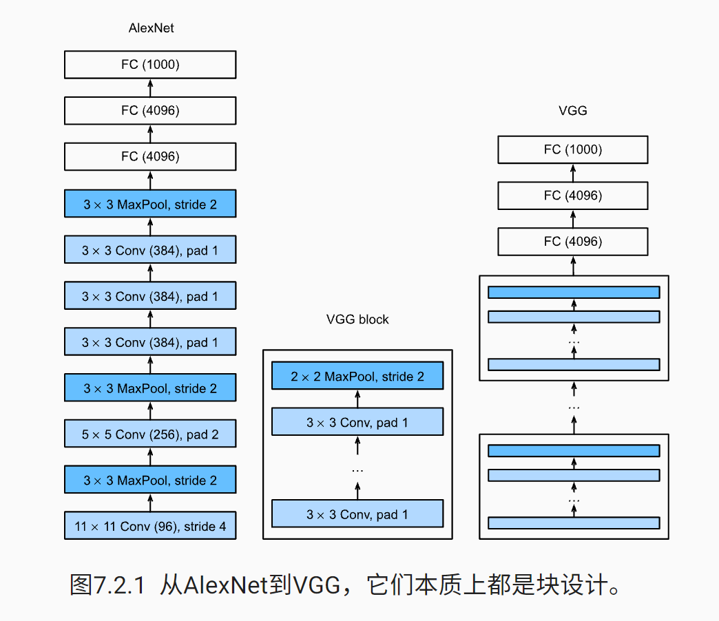
Several VGG blocks connected continuously by VGG neural network (defined in vgg_block function). There is a super parameter variable conv_arch . ** This variable specifies the number of convolution layers and output channels in each VGG block** The fully connected module is the same as in AlexNet.

conv_arch = ((1, 64), (1, 128), (2, 256), (2, 512), (2, 512))

The original VGG network has five convolution blocks, of which the first two blocks each have a convolution layer, and the last three blocks each contain two convolution layers. The first module has 64 output channels, and each subsequent module doubles the number of output channels until the number reaches 512. Since the network uses 8 convolution layers and 3 full connection layers, it is usually called VGG-11.

You can use conv_ Execute a for loop on arch to simply implement VGG-11.

def vgg(conv_arch):
    conv_blks = []
    in_channels = 1
    # Convolution layer part
    for (num_convs, out_channels) in conv_arch:
        conv_blks.append(vgg_block(num_convs, in_channels, out_channels))
        in_channels = out_channels

    return nn.Sequential(
        *conv_blks, nn.Flatten(),
        # Full connection layer
        nn.Linear(out_channels * 7 * 7, 4096), nn.ReLU(), nn.Dropout(0.5),
        nn.Linear(4096, 4096), nn.ReLU(), nn.Dropout(0.5),
        nn.Linear(4096, 10)
    )
net = vgg(conv_arch)

Next, we will build a single channel data sample with a height and width of 224 to observe the shape of the output of each layer.

X = torch.randn(size=(1, 1, 224, 224))
for blk in net:
    X = blk(X)
    print(blk.__class__.__name__,'output shape:\t',X.shape)
###########
Sequential output shape:     torch.Size([1, 64, 112, 112])
Sequential output shape:     torch.Size([1, 128, 56, 56])
Sequential output shape:     torch.Size([1, 256, 28, 28])
Sequential output shape:     torch.Size([1, 512, 14, 14])
Sequential output shape:     torch.Size([1, 512, 7, 7])
# Halve the height and width, and double the output channel
Flatten output shape:        torch.Size([1, 25088])
Linear output shape:         torch.Size([1, 4096])
ReLU output shape:   torch.Size([1, 4096])
Dropout output shape:        torch.Size([1, 4096])
Linear output shape:         torch.Size([1, 4096])
ReLU output shape:   torch.Size([1, 4096])
Dropout output shape:        torch.Size([1, 4096])
Linear output shape:         torch.Size([1, 10])

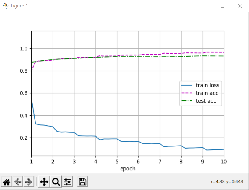
2.3. Training model

Since VGG-11 requires more computation than AlexNet, we built a network with fewer channels, which is enough to train the fashion MNIST dataset.

ratio = 4
small_conv_arch = [(pair[0], pair[1] // ratio) for pair in conv_arch]
net = vgg(small_conv_arch)

lr, num_epochs, batch_size = 0.05, 10, 128
train_iter, test_iter = d2l.load_data_fashion_mnist(batch_size, resize=224)
d2l.train_ch6(net, train_iter, test_iter, num_epochs, lr, d2l.try_gpu())

plt.show()

The following errors may occur:

RuntimeError: CUDA out of memory. Tried to allocate 98.00 MiB (GPU 0; 4.00 GiB total capacity; 
2.57 GiB already allocated; 0 bytes free; 2.67 GiB reserved in total by PyTorch)
(malloc at ..\c10\cuda\CUDACachingAllocator.cpp:289) (no backtrace available)

Action: reduce batch_size. batch_size = 64, 32, 16, etc.

2.4 summary

• VGG uses reusable convolution blocks to build a deep convolution network
• Different complexity variants can be obtained by different number of convolution blocks and hyperparameters

3. NiN Net in network

LeNet, AlexNet and VGG all have a common design pattern: extracting spatial structure features through a series of convolution layers and aggregation layers; Then the characterization of features is processed through the full connection layer.
AlexNet and VGG's improvement on LeNet mainly lies in how to expand and deepen these two modules. Alternatively, you can imagine using a full connection layer early in the process. However, if dense layers are used, the spatial structure of representation may be completely abandoned.
Network in network (NiN) provides a very simple solution: use multi-layer perceptron on each pixel channel.

Convolutional layers/Pooling layers/Dense Layer

3.1 NiN block

Recall that the inputs and outputs of the convolution layer are composed of four-dimensional tensors, and each axis of the tensor corresponds to the sample, channel, height and width respectively. In addition, the input and output of the full connection layer are usually two-dimensional tensors corresponding to samples and features respectively.

Here, let's think about how the convolution layer completes the work done by the full connection layer?
one × 1. Convolution
We can put 1 × 1 the convolution layer is regarded as a full connection layer applied at each pixel position, with c_i input values converted to c_o output values. Take the input as the input of the full connection layer, take any set of kernel functions as the weight, multiply and sum to obtain the output. (as like as two peas). From another perspective, each pixel in the spatial dimension is regarded as a single sample, and the channel dimension is regarded as different feature s.

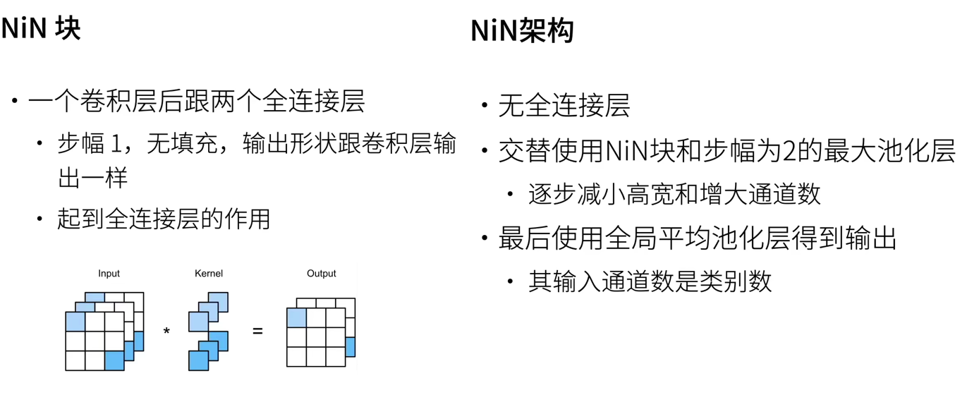
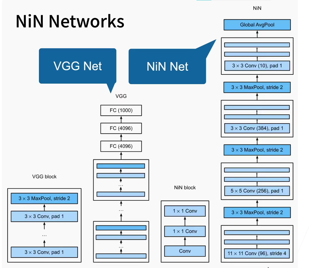
The NiN block starts with an ordinary convolution layer followed by two 1s × 1. These two 1 × 1 the convolution layer acts as a pixel by pixel full connection layer with ReLU activation function. The convolution window shape of the first layer is usually set by the user. The subsequent convolution window shape is fixed to 1 × 1 .

import torch
from torch import nn
from d2l import torch as d2l

def nin_block(in_channels, out_channels, kernel_size, strides, padding):
    return nn.Sequential(
        nn.Conv2d(in_channels, out_channels, kernel_size, strides, padding),
        nn.ReLU(),
        nn.Conv2d(out_channels, out_channels, kernel_size=1), nn.ReLU(),
        nn.Conv2d(out_channels, out_channels, kernel_size=1), nn.ReLU()
    )

3.2 NiN model

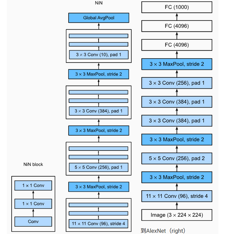
The window shape used by NiN is 11 × 11 , 5 × 5 and 3 × 3, the number of output channels is the same as that in AlexNet. There is a maximum convergence layer behind each NiN block, and the shape of the pool window is 3 × 3. The stride is 2.

A significant difference between NiN and AlexNet is that NiN completely cancels the full connection layer. Instead, NiN uses a NiN block with the number of output channels equal to the number of label categories. Finally, a global average pooling layer is placed to generate a multivariate logic vector (logits). One advantage of the NiN design is that it significantly reduces the number of parameters required for the model. However, in practice, this design sometimes increases the time of training the model.

net = nn.Sequential(
    nin_block(1, 96, kernel_size=11, strides=4, padding=0),
    nn.MaxPool2d(3, stride=2),
    nin_block(96, 256, kernel_size=5, strides=1, padding=2),
    nn.MaxPool2d(3, stride=2),
    nin_block(256, 384, kernel_size=3, strides=1, padding=1),
    nn.MaxPool2d(3, stride=2),
    nn.Dropout(0.5),
    # The number of label categories is 10
    nin_block(384, 10, kernel_size=3, strides=1, padding=1),
    nn.AdaptiveAvgPool2d((1, 1)),
    # Convert four-dimensional output into two-dimensional output in the shape of (batch size, 10)
    nn.Flatten())

X = torch.rand(size=(1, 1, 224, 224))
for layer in net:
    X = layer(X)
    print(layer.__class__.__name__,'output shape:\t', X.shape)
##############
Sequential output shape:	 torch.Size([1, 96, 54, 54])
MaxPool2d output shape:	 torch.Size([1, 96, 26, 26])
Sequential output shape:	 torch.Size([1, 256, 26, 26])
MaxPool2d output shape:	 torch.Size([1, 256, 12, 12])
Sequential output shape:	 torch.Size([1, 384, 12, 12])
MaxPool2d output shape:	 torch.Size([1, 384, 5, 5])
Dropout output shape:	 torch.Size([1, 384, 5, 5])
Sequential output shape:	 torch.Size([1, 10, 5, 5])
AdaptiveAvgPool2d output shape:	 torch.Size([1, 10, 1, 1])
Flatten output shape:	 torch.Size([1, 10])

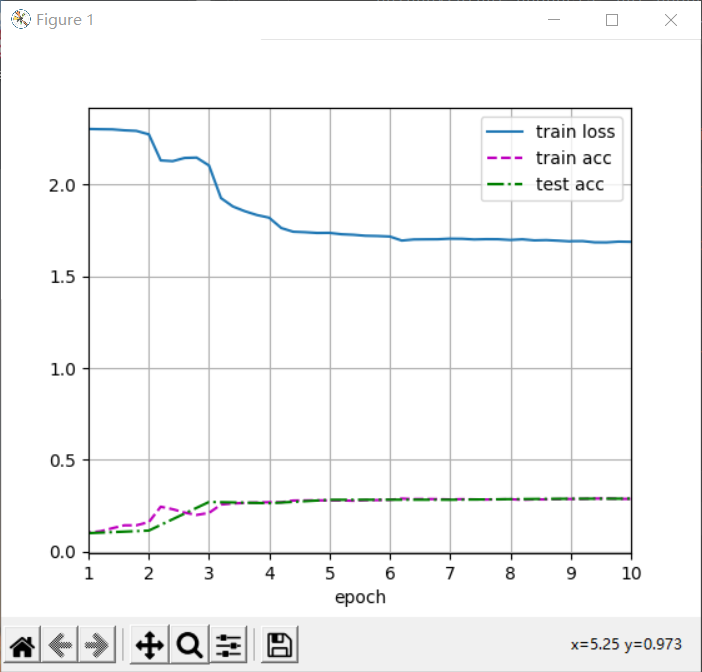
3.3 training model

As before, we used fashion MNIST to train the model. Training NiN is similar to training AlexNet and VGG.

lr, num_epochs, batch_size = 0.1, 10, 128
train_iter, test_iter = d2l.load_data_fashion_mnist(batch_size, resize=224)
d2l.train_ch6(net, train_iter, test_iter, num_epochs, lr, d2l.try_gpu())

plt.show()

3.4 summary

• The NiN block uses a convolution layer plus two 1x1 convolution layers, which adds nonlinearity to each pixel
• NiN uses the global average pooling layer to replace the full connection layer in VGG and AlexNet. It is not easy to over fit and has fewer parameters

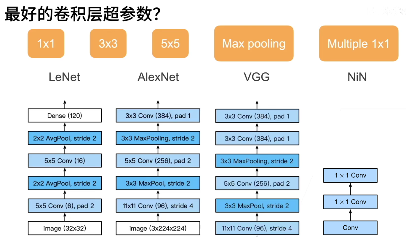
4. GoogLeNet with parallel connection

GoogLeNet absorbs the idea of serial network in NiN and makes improvements on this basis. A key point of this paper is to solve the problem of what size convolution kernel is the most suitable. After all, the popular Internet used to be as small as 1 × 1, up to 11 × Convolution kernel of 11. One view of this paper is that it is sometimes advantageous to use convolution kernel combinations of different sizes.

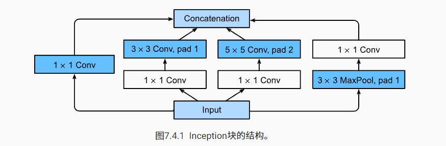
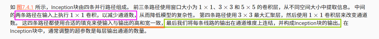
4.1 Inception block

In GoogLeNet, the basic convolution block is called an Inception block.

* args and * * kwargs in Python

import torch
from torch import nn
from torch.nn import functional as F
from d2l import torch as d2l

class Inception(nn.Module):
    def __init__(self, in_channels, c1, c2, c3, c4, **kwargs):
        super(Inception, self).__init__(**kwargs)
        self.p1_1 = nn.Conv2d(in_channels, c1, kernel_size=1)

        self.p2_1 = nn.Conv2d(in_channels, c2[0], kernel_size=1)
        self.p2_2 = nn.Conv2d(c2[0], c2[1], kernel_size=3, padding=1)

        self.p3_1 = nn.Conv2d(in_channels, c3[0], kernel_size=1)
        self.p3_2 = nn.Conv2d(c3[0], c3[1], kernel_size=5, padding=2)

        self.p4_1 = nn.MaxPool2d(kernel_size=3, stride=1, padding=1)
        self.p4_2 = nn.Conv2d(in_channels, c4, kernel_size=1)

    def  forward(self, x):
        p1 = F.relu(self.p1_1(x))
        p2 = F.relu(self.p2_2(F.relu(self.p2_1(x))))
        p3 = F.relu(self.p3_2(F.relu(self.p3_1(x))))
        p4 = F.relu(self.p4_2(self.p4_1(x)))
        return torch.cat((p1, p2, p3, p4), dim=1)

So why is GoogLeNet so effective? First, we consider the combination of filters, which can explore images with various filter sizes, which means that filters of different sizes can effectively identify different ranges of image details. At the same time, we can assign different numbers of parameters to different filters.

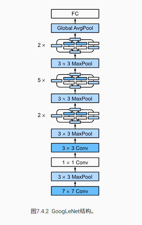
4.2 GoogLeNet model

GoogLeNet uses a total of 9 perception blocks and a stack of global average aggregation layers to generate its estimates. The maximum convergence layer between Inception blocks can reduce the dimension. The first module is similar to AlexNet and LeNet. The stack of Inception block is inherited from VGG. The global average aggregation layer avoids using the full connection layer at the end.

Now, let's implement each module of GoogLeNet one by one.

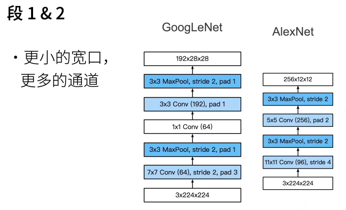
The first module uses 64 channels and 7 channels × 7. Convolution.

b1 = nn.Sequential(nn.Conv2d(1, 64, kernel_size=7, stride=2, padding=3),
                   nn.ReLU(),
                   nn.MaxPool2d(kernel_size=3, stride=2, padding=1))

The second module uses two convolution layers:
The first convolution layer is 64 channels, 1 × 1. Convolution layer;
The second convolution layer uses a 3-fold increase in the number of channels × 3. Convolution. This corresponds to the second path in the Inception block.

b2 = nn.Sequential(nn.Conv2d(64, 64, kernel_size=1),
                   nn.ReLU(),
                   nn.Conv2d(64, 192, kernel_size=3, padding=1),
                   nn.MaxPool2d(kernel_size=3, stride=2, padding=1))

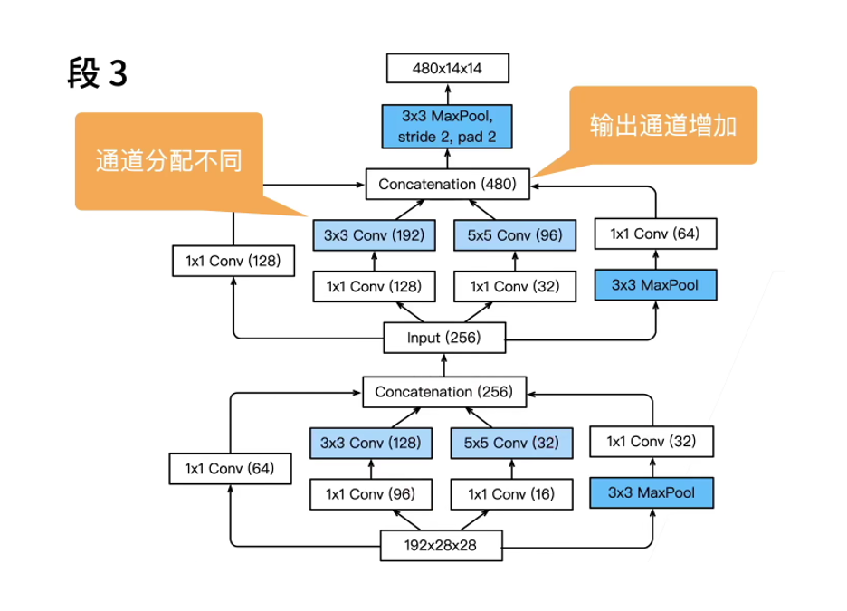
The third module connects two complete Inception blocks in series.
The number of output channels of the first Inception block is 64 + 128 + 32 + 32 = 256, and the number ratio of output channels between the four paths is 64:128:32:32 = 2:4:1:1. The second and third paths first reduce the number of input channels to 96 / 192 = 1 / 2 and 16 / 192 = 1 / 12, respectively, and then connect the second convolution layer.
The number of output channels of the second Inception block increases to 128 + 192 + 96 + 64 = 480 (the input of the next block), and the number ratio of output channels between the four paths is 128:192:96:64 = 4:6:3:2. The second and third paths first reduce the number of input channels to 128 / 256 = 1 / 2 and 32 / 256 = 1 / 8, respectively.

b3 = nn.Sequential(Inception(192, 64, (96, 128), (16, 32), 32),
                   Inception(256, 128, (128, 192), (32, 96), 64),
                   nn.MaxPool2d(kernel_size=3, stride=2, padding=1))

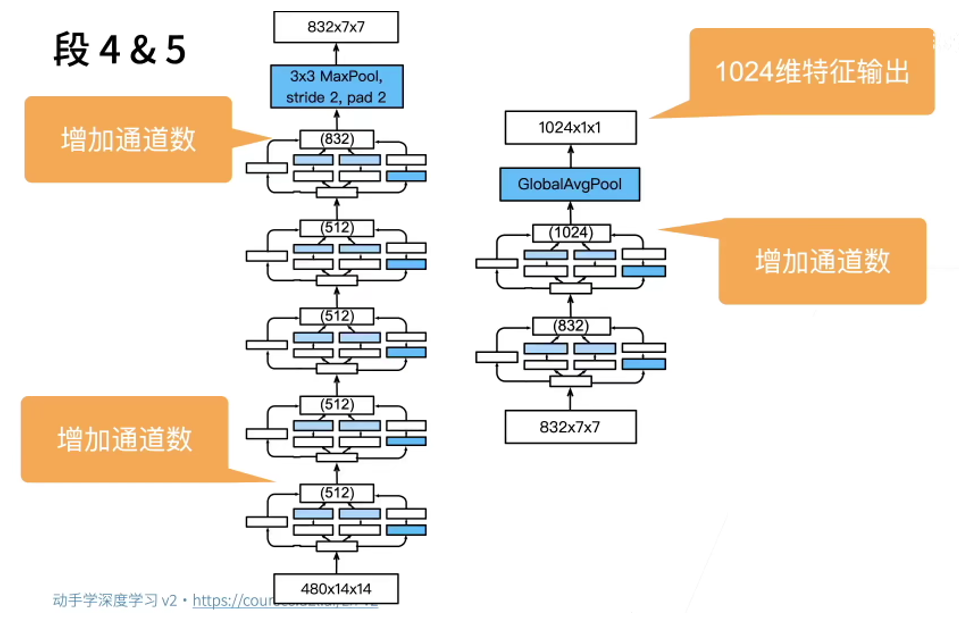
The fourth module is more complex. It connects five Inception blocks in series. The number of output channels are 192 + 208 + 48 + 64 = 512, 160 + 224 + 64 + 64 = 512, 128 + 256 + 64 + 64 = 512, 112 + 288 + 64 + 64 = 528 and 256 + 320 + 128 + 128 = 832 (the input of the next block). The channel number assignment of these paths is similar to that of the third module, and the first is 3. × The second path of 3 convolution layer outputs the most channels, followed by only 1 × The first path of 1 convolution, followed by 5 × The third path of the 5 convolution layer and including 3 × 3. The fourth path of the maximum convergence layer. The second and third paths will first reduce the number of channels in proportion. These scales vary slightly in each Inception block.

b4 = nn.Sequential(Inception(480, 192, (96, 208), (16, 48), 64),
                   Inception(512, 160, (112, 224), (24, 64), 64),
                   Inception(512, 128, (128, 256), (24, 64), 64),
                   Inception(512, 112, (144, 288), (32, 64), 64),
                   Inception(528, 256, (160, 320), (32, 128), 128),
                   nn.MaxPool2d(kernel_size=3, stride=2, padding=1))

The fifth module includes two Inception blocks with the number of output channels of 256 + 320 + 128 + 128 = 832 and 384 + 384 + 128 + 128 = 1024. The allocation idea of the number of channels in each path is the same as that in the third and fourth modules, but the specific values are different. It should be noted that the fifth module is followed by the output layer. Like NiN, this module uses the global average aggregation layer to change the height and width of each channel to 1. Finally, we turn the output into a two-dimensional array, and then connect a full connection layer whose output number is the number of label categories.

b5 = nn.Sequential(Inception(832, 256, (160, 320), (32, 128), 128),
                   Inception(832, 384, (192, 384), (48, 128), 128),
                   nn.AdaptiveAvgPool2d((1,1)),
                   nn.Flatten())

net = nn.Sequential(b1, b2, b3, b4, b5, nn.Linear(1024, 10))

4.3 training model

As before, we used the fashion MNIST dataset to train our model. Before training, we convert the picture to 96 × 96 resolution.

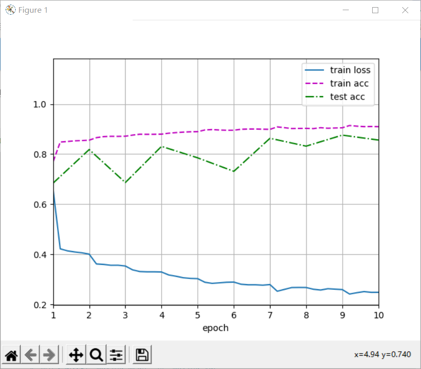
lr, num_epochs, batch_size = 0.1, 10, 128
train_iter, test_iter = d2l.load_data_fashion_mnist(batch_size, resize=96)
d2l.train_ch6(net, train_iter, test_iter, num_epochs, lr, d2l.try_gpu())

plt.show()

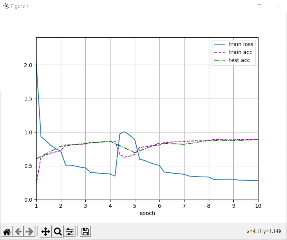
loss 0.281, train acc 0.892, test acc 0.890
733.0 examples/sec on cuda:0

4.4 summary

• The Inception block uses four convolution layer and pooling layer paths with different superparameters to extract different information, and uses 1 × 1 the convolution layer reduces the channel dimension at the per pixel level, thereby reducing the model complexity.
• GoogLeNet connects several finely designed concept blocks with other layers (convolution layer, full connection layer). The channel number allocation ratio of the Inception block is obtained through a large number of experiments on the ImageNet dataset.

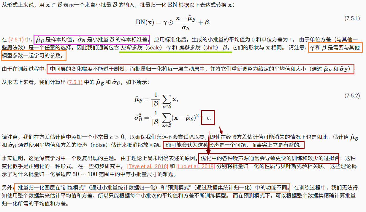
5 batch normalization

It is very difficult to train deep neural networks, especially to make them converge in a short time. Batch normalization can continuously accelerate the convergence speed of deep network. Combined with the residual block to be introduced soon, batch normalization enables researchers to train networks with more than 100 layers.

5.1 training deep network

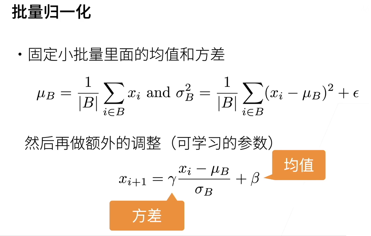
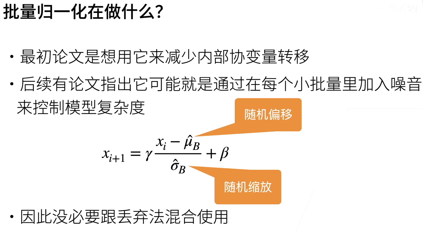
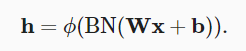
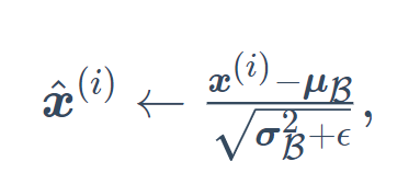
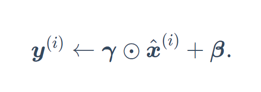
Batch normalization is applied to a single optional layer (or all layers). Its principle is as follows: in each training iteration, we first normalize the input, that is, by subtracting its mean value and dividing it by its standard deviation, both of which are based on the current small batch processing. Next, we apply a scale factor and a scale offset. It is this standardization based on batch statistics that gives the name of batch normalization.

Please note that if we try to apply batch normalization with a small batch of size 1, we will not learn anything. This is because after subtracting the mean, each hidden cell will be 0. Therefore, batch normalization is effective and stable only when a large enough small batch is used. Note that when applying batch normalization, the selection of batch size may be more important than when there is no batch normalization.

5.2 batch normalization layer

Batch normalization runs on complete small batches, so we can't ignore the size of the batch as before when introducing other layers. We discuss these two cases below: full connection layer and convolution layer.

5.2.1 full connection layer

The batch normalization layer is placed between the affine transformation and the activation function in the full connection layer. Let the input of the full connection layer be u, the weight parameters and offset parameters be W and b respectively, and the activation function be ϕ ， The operator of batch normalization is BN.

5.2.2 convolution

For convolution layers, batch normalization can be applied after the convolution layer and before the nonlinear activation function. When the convolution has multiple output channels, we need to perform batch normalization on the "each" output of these channels, and each channel has its own scale and shift parameters.

5.2.3 batch normalization during prediction

Batch normalization usually behaves differently in training mode and prediction mode. Firstly, when the trained model is used for prediction, we no longer need the noise in the sample mean and the sample variance generated by each small batch on the micro batch. Second, for example, we may need to use our model to predict sample by sample. A common method is to estimate the sample mean and variance of the whole training data set by moving average, and use them to obtain the determined output. It can be seen that, like dropout, the calculation results of batch normalization layer in training mode and prediction mode are also different.

5.3 summary

• Batch normalization fixes the mean and variance in a small batch, and then learns the appropriate offset and scaling
• It can accelerate the convergence speed, but generally does not change the accuracy of the model

5.4 implementation from zero

The following function implements the specific function steps of batch normalization, which does not involve the design of layers.

def batch_norm(X, gamma, beta, moving_mean, moving_var, eps, momentum):
    # Via ` is_grad_enabled ` to judge whether the current mode is training mode or prediction mode
    if not torch.is_grad_enabled():
        # If it is in the prediction mode, the mean and variance obtained by the incoming moving average are directly used
        # moving_mean,moving_var is the global mean and variance
        X_hat = (X - moving_mean) / torch.sqrt(moving_var + eps)
    else:
        assert len(X.shape) in (2, 4)
        if len(X.shape) == 2:  # If it is two-dimensional, the first dimension is the batch size (number of samples), and the second dimension is the feature
            # In the case of full connection layer, the mean and variance on the feature dimension are calculated
            mean = X.mean(dim=0)  # Calculate the mean value for each column, that is, calculate the mean value for each feature
            var = ((X - mean) ** 2).mean(dim=0)
        else:  # If it is 4-dimensional, the first dimension is batch size (number of samples), and the third and fourth dimensions are width and height
            # Using the case of two-dimensional convolution, calculate the mean and variance on the channel dimension (axis=1).
            # Here we need to keep the shape of X so that we can do broadcast operation later
            mean = X.mean(dim=(0, 2, 3), keepdim=True)
            var = ((X - mean) ** 2).mean(dim=(0, 2, 3), keepdim=True)
        # In the training mode, the current mean and variance are used for standardization
        X_hat = (X - mean) / torch.sqrt(var + eps)
        # Update the mean and variance of the moving average
        moving_mean = momentum * moving_mean + (1.0 - momentum) * mean
        moving_var = momentum * moving_var + (1.0 - momentum) * var
    Y = gamma * X_hat + beta  # Scaling and shifting
    return Y, moving_mean.data, moving_var.data

You can now create a correct BatchNorm layer. This layer will maintain appropriate parameters: stretch gamma and offset beta, which will be updated during training. In addition, our layer will save the moving average of mean and variance for subsequent use during model prediction.

Note that we implement the basic design pattern of layers. Usually, we use a single function to define its mathematical principle, such as batch_norm. Then, we integrate this function into a custom layer,

class BatchNorm(nn.Module):
    # `num_features `: the number of outputs of the fully connected layer or the number of output channels of the convolution layer.
    # `num_dims `: 2 indicates the fully connected layer and 4 indicates the convolution layer
    def __init__(self, num_features, num_dims):
        super().__init__()
        if num_dims == 2:
            shape = (1, num_features)
        else:
            shape = (1, num_features, 1, 1)
        # Stretch and offset parameters involved in gradient and iteration are initialized to 1 and 0 respectively
        self.gamma = nn.Parameter(torch.ones(shape))
        self.beta = nn.Parameter(torch.zeros(shape))
        # Variables that are not model parameters are initialized to 0 and 1
        self.moving_mean = torch.zeros(shape)
        self.moving_var = torch.ones(shape)

    def forward(self, X):
        # If 'X' is not in memory, it will be 'moving'_ Mean ` and ` moving_var`
        # Copy to the video memory where 'X' is located
        if self.moving_mean.device != X.device:
            self.moving_mean = self.moving_mean.to(X.device)
            self.moving_var = self.moving_var.to(X.device)
        # Save updated ` moving_mean ` and ` moving_var`
        Y, self.moving_mean, self.moving_var = batch_norm(
            X, self.gamma, self.beta, self.moving_mean,
            self.moving_var, eps=1e-5, momentum=0.9)
        return Y

5.5 LeNet using batch normalization layer

To better understand how to apply BatchNorm, let's apply it to the LeNet model. Recall that batch normalization is applied after the convolution layer or full connection layer and before the corresponding activation function.

net = nn.Sequential(
    nn.Conv2d(1, 6, kernel_size=5), BatchNorm(6, num_dims=4), nn.Sigmoid(),
    nn.MaxPool2d(kernel_size=2, stride=2),
    nn.Conv2d(6, 16, kernel_size=5), BatchNorm(16, num_dims=4), nn.Sigmoid(),
    nn.MaxPool2d(kernel_size=2, stride=2), 
    nn.Flatten(),
    nn.Linear(16*4*4, 120), BatchNorm(120, num_dims=2), nn.Sigmoid(),
    nn.Linear(120, 84), BatchNorm(84, num_dims=2), nn.Sigmoid(),
    nn.Linear(84, 10))

lr, num_epochs, batch_size = 1.0, 10, 256
train_iter, test_iter = d2l.load_data_fashion_mnist(batch_size)
d2l.train_ch6(net, train_iter, test_iter, num_epochs, lr, d2l.try_gpu())

plt.show()

This code is almost the same as when we first trained LeNet. The main difference is that the learning rate is much higher.

loss 0.248, train acc 0.910, test acc 0.856
19017.5 examples/sec on cuda:0

You can see the stretching parameter gamma and offset parameter beta learned from the first batch normalization layer.

print(net[1].gamma.reshape((-1,)), net[1].beta.reshape((-1,)))
##############################
tensor([1.6943, 1.8941, 2.5112, 1.5086, 2.3657, 2.2883], device='cuda:0',
       grad_fn=<ViewBackward>) tensor([ 0.1875,  0.8067, -2.6232, -0.9846, -0.4181, -0.1513], device='cuda:0',
       grad_fn=<ViewBackward>)

5.6 concise implementation

BatchNorm2d: applies to the volume layer.
BatchNorm1d: applies to the full connection layer.

It is equivalent to the batch we implemented above_ Normal function and BatchNorm layer.

net = nn.Sequential(
    nn.Conv2d(1, 6, kernel_size=5), nn.BatchNorm2d(6), nn.Sigmoid(),
    nn.MaxPool2d(kernel_size=2, stride=2),
    nn.Conv2d(6, 16, kernel_size=5), nn.BatchNorm2d(16), nn.Sigmoid(),
    nn.MaxPool2d(kernel_size=2, stride=2), nn.Flatten(),
    nn.Linear(256, 120), nn.BatchNorm1d(120), nn.Sigmoid(),
    nn.Linear(120, 84), nn.BatchNorm1d(84), nn.Sigmoid(),
    nn.Linear(84, 10))

d2l.train_ch6(net, train_iter, test_iter, num_epochs, lr, d2l.try_gpu())

Training data set	Forecast data set
Noise needs to be added	The noise in the sample mean is no longer needed
Mean and variance in small batch	Mean and variance of all data

6 residual network ResNet

As we design deeper and deeper networks, it is very important to deeply understand "how the newly added layer improves the performance of neural networks". More important is the ability to design networks.

6.1 function class

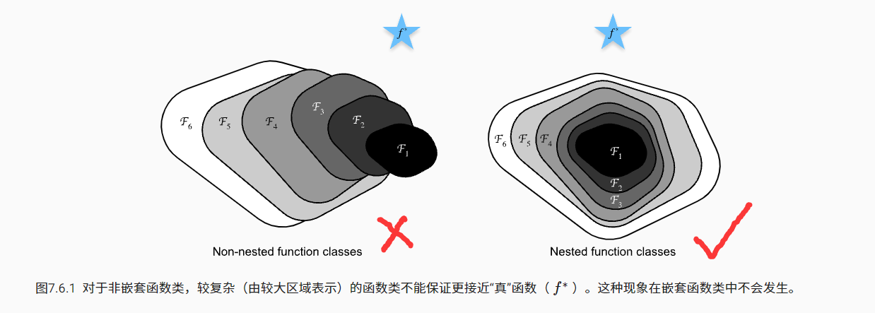
Therefore, only when more complex function classes contain smaller function classes can we ensure that their performance is improved. For deep neural networks, if we can train the newly added layer into identity function f(x)=x, the new model and the original model will be equally effective. At the same time, because the new model may get a better solution to fit the training data set, it seems easier to reduce the training error by adding layers.

The core idea of residual network is that each additional layer should more easily contain the original function as one of its elements. Thus, residual blocks were born. This design has a far-reaching impact on how to establish deep neural networks.

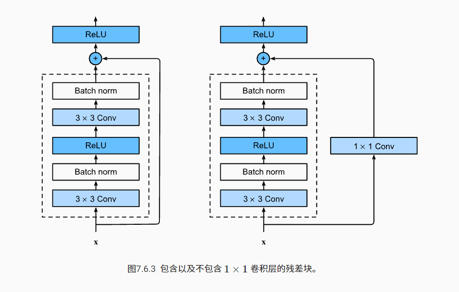
6.2 residual block

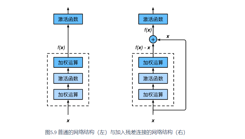
The part in the dotted box on the left needs to fit the mapping f(x) directly, while the part in the dotted box on the right needs to fit the residual mapping f(x) − X. Residual mapping is often easier to optimize in reality.

If you want to change the number of channels, you need to introduce an additional 1 × 1 convolution layer to transform the input into the desired shape before adding.

import torch
from torch import nn
from torch.nn import functional as F
from d2l import torch as d2l

class Residual(nn.Module):
    def __init__(self, input_channels, num_channels,
                 use_1x1conv=False, strides=1):
        # ResNet follows VGG's complete 3 × 3 convolution design, there are first 2 3 with the same number of output channels in the residual block × 3 convolution
        self.conv1 = nn.Conv2d(input_channels, num_channels,
                               kernel_size=3, padding=1, stride=strides)
        self.conv2 = nn.Conv2d(num_channels, num_channels,
                               kernel_size=3, padding=1)
        if use_1x1conv:
            self.conv3 = nn.Conv2d(input_channels, num_channels,
                                   kernel_size=1, stride=strides)
        else:
            self.conv3 = None
        self.bn1 = nn.BatchNorm2d(num_channels)
        self.bn2 = nn.BatchNorm2d(num_channels)
        self.relu = nn.ReLU(inplace=True)

    def forward(self, X):
        Y = F.relu(self.bn1(self.conv1(X)))
        Y = self.bn2(self.conv2(Y))
        if self.conv3:
            X = self.conv3(X)
        Y += X
        return F.relu(Y)

This code generates two types of networks:
One is in use_1x1conv=False, add input to output before applying ReLU nonlinear function.
The other is in use_ When 1x1conv = true, add 1 × 1. Adjust the channel and resolution.

View the consistency of input and output shapes.

blk = Residual(3, 3)  # The first is the input channel and the second is the output channel
print(blk)
X = torch.rand(4, 3, 6, 6)  # Batch size, number of channels, height, width
Y = blk(X)
print(Y.shape)
##############
Residual(
  (conv1): Conv2d(3, 3, kernel_size=(3, 3), stride=(1, 1), padding=(1, 1))
  (conv2): Conv2d(3, 3, kernel_size=(3, 3), stride=(1, 1), padding=(1, 1))
  (bn1): BatchNorm2d(3, eps=1e-05, momentum=0.1, affine=True, track_running_stats=True)
  (bn2): BatchNorm2d(3, eps=1e-05, momentum=0.1, affine=True, track_running_stats=True)
  (relu): ReLU(inplace=True)
)
torch.Size([4, 3, 6, 6])

We can also increase the number of output channels and halve the output height and width.

blk = Residual(3, 6, use_1x1conv=True, strides=2)
print(blk(X).shape)
########
torch.Size([4, 6, 3, 3])

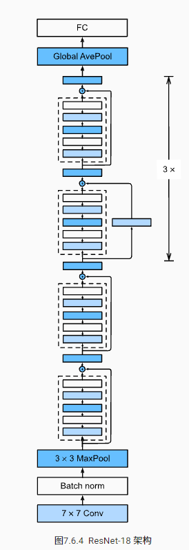
6.3 ResNet model

The first two layers of ResNet are the same as those in GoogLeNet: 7 with 64 output channels and 2 steps × 7 after the convolution, follow the 3 with a step of 2 × 3 Maximum convergence layer. The difference is that ResNet adds a batch normalization layer after each convolution layer.

b1 = nn.Sequential(nn.Conv2d(1, 64, kernel_size=7, stride=2, padding=3),
                   nn.BatchNorm2d(64), nn.ReLU(),
                   nn.MaxPool2d(kernel_size=3, stride=2, padding=1))

GoogLeNet is followed by four modules composed of Inception blocks. ResNet uses four modules composed of residual blocks, and each module uses several residual blocks with the same number of output channels.

def resnet_block(input_channels, num_channels, num_residuals,
                 first_block=False):
    blk = []
    for i in range(num_residuals):
        if i == 0 and not first_block:
            blk.append(Residual(input_channels, num_channels,
                                use_1x1conv=True, strides=2))
        else:
            blk.append(Residual(num_channels, num_channels))
    return blk

Then add all residual blocks in ResNet, where each module uses 2 residual blocks.

b2 = nn.Sequential(*resnet_block(64, 64, 2, first_block=True))
b3 = nn.Sequential(*resnet_block(64, 128, 2))
b4 = nn.Sequential(*resnet_block(128, 256, 2))
b5 = nn.Sequential(*resnet_block(256, 512, 2))

Finally, like GoogLeNet, the global average aggregation layer and full connection layer output are added to ResNet.

net = nn.Sequential(b1, b2, b3, b4, b5,
                    nn.AdaptiveAvgPool2d((1,1)),
                    nn.Flatten(), nn.Linear(512, 10))

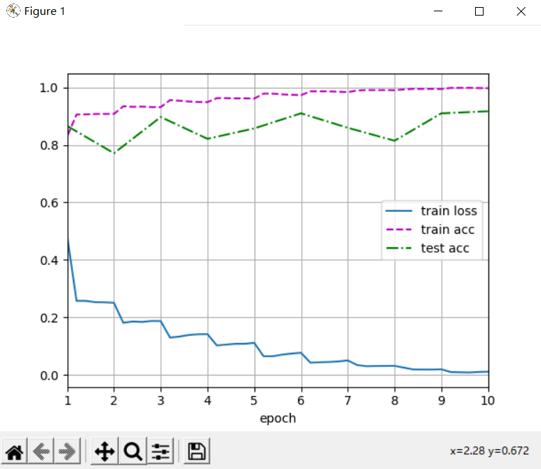
6.4 training model

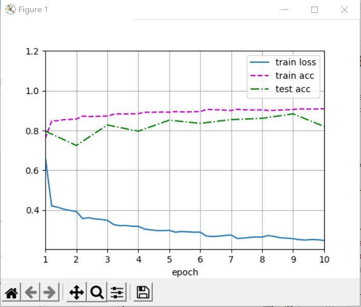
lr, num_epochs, batch_size = 0.05, 10, 256
train_iter, test_iter = d2l.load_data_fashion_mnist(batch_size, resize=96)
d2l.train_ch6(net, train_iter, test_iter, num_epochs, lr, d2l.try_gpu())

plt.show()

6.5 summary

• Residual blocks make deep networks easier to train
• Residual network has a far-reaching impact on the subsequent deep neural network design, whether convolution network or fully connected network
• The original paper said that the gradient explosion and gradient disappearance are basically solved after the introduction of bn layer, and the residual is to solve the network degradation