Three methods of initializing parameters
First, download the data set and necessary files required for this practice. ( Download link )Put it in the project folder established below.

Then open pycharm, create a new project called improved neural network, and then create a new python file called init.py. Three initialization methods are used to import related libraries and data sets, namely zero initialization, random initialization, and He initialization.
Zero initialization: set in the input parameters initialization = "zeros".
Random initialization: set in the input parameters initialization = "random"
He Initialization: set in input parameters initialization = "he"
Finally, the codes of the three initialization methods are as follows. You can cancel the annotation of the training model code under a method to view the training effect of the method. Only the effect of the last He initialization is shown here.
# Import the required libraries and datasets
import numpy as np
import matplotlib.pyplot as plt
import sklearn
import sklearn.datasets
import init_utils #Part I, initialization
import reg_utils #The second part is regularization
import gc_utils #The third part is gradient verification
from init_utils import sigmoid, relu, compute_loss, forward_propagation, backward_propagation
from init_utils import update_parameters, predict, load_dataset, plot_decision_boundary, predict_dec
# set default size of plots
plt.rcParams['figure.figsize'] = (7.0, 4.0)
plt.rcParams['image.interpolation'] = 'nearest'
plt.rcParams['image.cmap'] = 'gray'
# Read and draw data
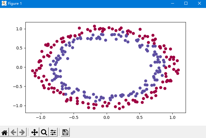
train_X, train_Y, test_X, test_Y = load_dataset()
#Drawing display
# plt.show()
# Define neural network model
def model(X, Y, learning_rate=0.01, num_iterations=15000, print_cost=True, initialization="he", is_polt=True):
"""
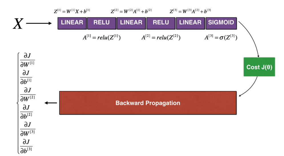
Implement a three-layer neural network: LINEAR ->RELU -> LINEAR -> RELU -> LINEAR -> SIGMOID
Parameters:
X - The dimension of the entered data is(2, To train/Number of tests)
Y - Label, [0] | 1],Dimension is(1,This corresponds to the label of the input data)
learning_rate - Learning rate
num_iterations - Number of iterations
print_cost - Print cost value, once every 1000 iterations
initialization - String type, initialization type["zeros" | "random" | "he"]
is_polt - Whether to draw the curve of gradient descent
return
parameters - Parameters after learning
"""
grads = {}
costs = []
m = X.shape[1]
layers_dims = [X.shape[0], 10, 5, 1]
# Select the type of initialization parameter
if initialization == "zeros":
parameters = initialize_parameters_zeros(layers_dims)
elif initialization == "random":
parameters = initialize_parameters_random(layers_dims)
elif initialization == "he":
parameters = initialize_parameters_he(layers_dims)
else:
print("Bad initialization parameters! Program exit")
exit
# Start learning
for i in range(0, num_iterations):
# Forward propagation
a3, cache = init_utils.forward_propagation(X, parameters)
# Calculate cost
cost = init_utils.compute_loss(a3, Y)
# Back propagation
grads = init_utils.backward_propagation(X, Y, cache)
# Update parameters
parameters = init_utils.update_parameters(parameters, grads, learning_rate)
# Record cost
if i % 1000 == 0:
costs.append(cost)
# Print cost
if print_cost:
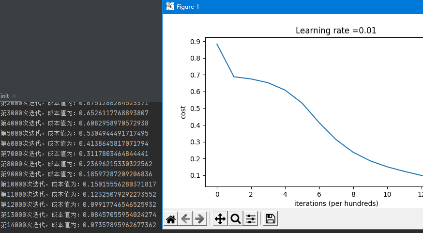
print("The first" + str(i) + "For the second iteration, the cost value is:" + str(cost))
# After learning, draw the cost curve
if is_polt:
plt.plot(costs)
plt.ylabel('cost')
plt.xlabel('iterations (per hundreds)')
plt.title("Learning rate =" + str(learning_rate))
plt.show()
# Return parameters after learning
return parameters
# All parameters are initialized to 0
def initialize_parameters_zeros(layers_dims):
"""
Set all parameters of the model to 0
Parameters:
layers_dims - List, the number of layers of the model and the number of nodes corresponding to each layer
return
parameters - Contains all W and b Dictionary of
W1 - Weight matrix, dimension( layers_dims[1], layers_dims[0])
b1 - Offset vector, dimension( layers_dims[1],1)
···
WL - Weight matrix, dimension( layers_dims[L], layers_dims[L -1])
bL - Offset vector, dimension( layers_dims[L],1)
"""
parameters = {}
L = len(layers_dims) # Number of network layers
for l in range(1, L):
parameters["W" + str(l)] = np.zeros((layers_dims[l], layers_dims[l - 1]))
parameters["b" + str(l)] = np.zeros((layers_dims[l], 1))
assert (parameters["W" + str(l)].shape == (layers_dims[l], layers_dims[l - 1]))
assert (parameters["b" + str(l)].shape == (layers_dims[l], 1))
return parameters
# Test to see if they are all 0
# parameters = initialize_parameters_zeros([3,2,1])
# print("W1 = " + str(parameters["W1"]))
# print("b1 = " + str(parameters["b1"]))
# print("W2 = " + str(parameters["W2"]))
# print("b2 = " + str(parameters["b2"]))
# The training model is initialized with zero
#parameters = model(train_X, train_Y, initialization="zeros",is_polt=True)
#View forecast results
#print ("training set:")
#predictions_train = init_utils.predict(train_X, train_Y, parameters)
#print ("test set:")
#predictions_test = init_utils.predict(test_X, test_Y, parameters)
# Parameter random initialization
def initialize_parameters_random(layers_dims):
"""
Parameters:
layers_dims - List, the number of layers of the model and the number of nodes corresponding to each layer
return
parameters - Contains all W and b Dictionary of
W1 - Weight matrix, dimension( layers_dims[1], layers_dims[0])
b1 - Offset vector, dimension( layers_dims[1],1)
···
WL - Weight matrix, dimension( layers_dims[L], layers_dims[L -1])
b1 - Offset vector, dimension( layers_dims[L],1)
Initialize weights to larger random values (press*10 Zoom) and set the deviation to 0.
take np.random.randn(..,..) * 10 For weights, set np.zeros((.., ..))For deviation
"""
parameters = {}
L = len(layers_dims) # Number of layers
for l in range(1, L):
parameters['W' + str(l)] = np.random.randn(layers_dims[l], layers_dims[l - 1]) * 10 # Use 10x zoom
parameters['b' + str(l)] = np.zeros((layers_dims[l], 1))
# Use assertions to ensure that my data format is correct
assert (parameters["W" + str(l)].shape == (layers_dims[l], layers_dims[l - 1]))
assert (parameters["b" + str(l)].shape == (layers_dims[l], 1))
return parameters
# Test the parameter output of random initialization
# parameters = initialize_parameters_random([3, 2, 1])
# print("W1 = " + str(parameters["W1"]))
# print("b1 = " + str(parameters["b1"]))
# print("W2 = " + str(parameters["W2"]))
# print("b2 = " + str(parameters["b2"]))
#Use random initialization training model
#parameters = model(train_X, train_Y, initialization = "random",is_polt=True)
#Output the accuracy of training set and test set
# print("training set:")
# predictions_train = init_utils.predict(train_X, train_Y, parameters)
# print("test set:")
# predictions_test = init_utils.predict(test_X, test_Y, parameters)
# View the classification results of the graph
# plt.title("Model with large random initialization")
# axes = plt.gca()
# axes.set_xlim([-1.5, 1.5])
# axes.set_ylim([-1.5, 1.5])
# init_utils.plot_decision_boundary(lambda x: init_utils.predict_dec(parameters, x.T), train_X, train_Y)
# He initialization, according to the paper of he et al
def initialize_parameters_he(layers_dims):
"""
Parameters:
layers_dims - List, the number of layers of the model and the number of nodes corresponding to each layer
return
parameters - Contains all W and b Dictionary of
W1 - Weight matrix, dimension( layers_dims[1], layers_dims[0])
b1 - Offset vector, dimension( layers_dims[1],1)
···
WL - Weight matrix, dimension( layers_dims[L], layers_dims[L -1])
b1 - Offset vector, dimension( layers_dims[L],1)
"""
np.random.seed(3) # Specify random seed
parameters = {}
L = len(layers_dims) # Number of layers
for l in range(1, L):
parameters['W' + str(l)] = np.random.randn(layers_dims[l], layers_dims[l - 1]) * np.sqrt(2 / layers_dims[l - 1])
parameters['b' + str(l)] = np.zeros((layers_dims[l], 1))
# Use assertions to ensure that my data format is correct
assert (parameters["W" + str(l)].shape == (layers_dims[l], layers_dims[l - 1]))
assert (parameters["b" + str(l)].shape == (layers_dims[l], 1))
return parameters
# Train the model and output the accuracy of the model
parameters = model(train_X, train_Y, initialization = "he",is_polt=True)
#
#
print("Training set:")
predictions_train = init_utils.predict(train_X, train_Y, parameters)
print("Test set:")
init_utils.predictions_test = init_utils.predict(test_X, test_Y, parameters)
# Draw a picture of the forecast
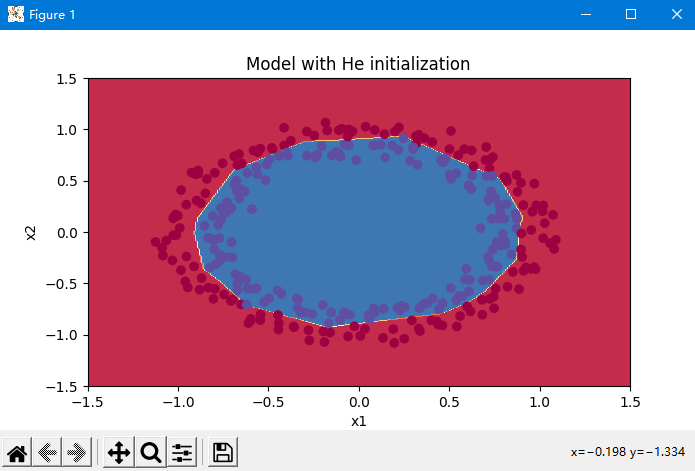
plt.title("Model with He initialization")
axes = plt.gca()
axes.set_xlim([-1.5, 1.5])
axes.set_ylim([-1.5, 1.5])
init_utils.plot_decision_boundary(lambda x: init_utils.predict_dec(parameters, x.T), train_X, train_Y)
The data initially loaded is shown below,
Using the method of He, the cost function J is as follows
Final classification effect
Initialization weight parameter complete code
# Import the required libraries and datasets
import numpy as np
import matplotlib.pyplot as plt
import sklearn
import sklearn.datasets
import init_utils   #Part I, initialization
import reg_utils    #The second part is regularization
import gc_utils     #The third part is gradient verification
from init_utils import sigmoid, relu, compute_loss, forward_propagation, backward_propagation
from init_utils import update_parameters, predict, load_dataset, plot_decision_boundary, predict_dec

# set default size of plots
plt.rcParams['figure.figsize'] = (7.0, 4.0)
plt.rcParams['image.interpolation'] = 'nearest'
plt.rcParams['image.cmap'] = 'gray'
# Read and draw data
train_X, train_Y, test_X, test_Y = load_dataset()
#Drawing display
plt.show()

# Define neural network model
def model(X, Y, learning_rate=0.01, num_iterations=15000, print_cost=True, initialization="he", is_polt=True):
    """
    Implement a three-layer neural network: LINEAR ->RELU -> LINEAR -> RELU -> LINEAR -> SIGMOID

    Parameters:
        X - The dimension of the entered data is(2, To train/Number of tests)
        Y - Label, [0] | 1],Dimension is(1,This corresponds to the label of the input data)
        learning_rate - Learning rate
        num_iterations - Number of iterations
        print_cost - Print cost value, once every 1000 iterations
        initialization - String type, initialization type["zeros" | "random" | "he"]
        is_polt - Whether to draw the curve of gradient descent
    return
        parameters - Parameters after learning
    """
    grads = {}
    costs = []
    m = X.shape[1]
    layers_dims = [X.shape[0], 10, 5, 1]

    # Select the type of initialization parameter
    if initialization == "zeros":
        parameters = initialize_parameters_zeros(layers_dims)
    elif initialization == "random":
        parameters = initialize_parameters_random(layers_dims)
    elif initialization == "he":
        parameters = initialize_parameters_he(layers_dims)
    else:
        print("Bad initialization parameters! Program exit")
        exit

    # Start learning
    for i in range(0, num_iterations):
        # Forward propagation
        a3, cache = init_utils.forward_propagation(X, parameters)

        # Calculate cost
        cost = init_utils.compute_loss(a3, Y)

        # Back propagation
        grads = init_utils.backward_propagation(X, Y, cache)

        # Update parameters
        parameters = init_utils.update_parameters(parameters, grads, learning_rate)

        # Record cost
        if i % 1000 == 0:
            costs.append(cost)
            # Print cost
            if print_cost:
                print("The first" + str(i) + "For the second iteration, the cost value is:" + str(cost))

    # After learning, draw the cost curve
    if is_polt:
        plt.plot(costs)
        plt.ylabel('cost')
        plt.xlabel('iterations (per hundreds)')
        plt.title("Learning rate =" + str(learning_rate))
        plt.show()

    # Return parameters after learning
    return parameters


# All parameters are initialized to 0
def initialize_parameters_zeros(layers_dims):
    """
    Set all parameters of the model to 0

    Parameters:
        layers_dims - List, the number of layers of the model and the number of nodes corresponding to each layer
    return
        parameters - Contains all W and b Dictionary of
            W1 - Weight matrix, dimension( layers_dims[1], layers_dims[0])
            b1 - Offset vector, dimension( layers_dims[1],1)
            ···
            WL - Weight matrix, dimension( layers_dims[L], layers_dims[L -1])
            bL - Offset vector, dimension( layers_dims[L],1)
    """
    parameters = {}

    L = len(layers_dims)  # Number of network layers

    for l in range(1, L):
        parameters["W" + str(l)] = np.zeros((layers_dims[l], layers_dims[l - 1]))
        parameters["b" + str(l)] = np.zeros((layers_dims[l], 1))

    assert (parameters["W" + str(l)].shape == (layers_dims[l], layers_dims[l - 1]))
    assert (parameters["b" + str(l)].shape == (layers_dims[l], 1))

    return parameters

# Test to see if they are all 0
# parameters = initialize_parameters_zeros([3,2,1])
# print("W1 = " + str(parameters["W1"]))
# print("b1 = " + str(parameters["b1"]))
# print("W2 = " + str(parameters["W2"]))
# print("b2 = " + str(parameters["b2"]))

# The training model is initialized with zero
#parameters = model(train_X, train_Y, initialization="zeros",is_polt=True)


#View forecast results
#print ("training set:")
#predictions_train = init_utils.predict(train_X, train_Y, parameters)
#print ("test set:")
#predictions_test = init_utils.predict(test_X, test_Y, parameters)

# Parameter random initialization
def initialize_parameters_random(layers_dims):
    """
    Parameters:
        layers_dims - List, the number of layers of the model and the number of nodes corresponding to each layer
    return
        parameters - Contains all W and b Dictionary of
            W1 - Weight matrix, dimension( layers_dims[1], layers_dims[0])
            b1 - Offset vector, dimension( layers_dims[1],1)
            ···
            WL - Weight matrix, dimension( layers_dims[L], layers_dims[L -1])
            b1 - Offset vector, dimension( layers_dims[L],1)
            Initialize weights to larger random values (press*10 Zoom) and set the deviation to 0.
            take np.random.randn(..,..) * 10 For weights, set np.zeros((.., ..))For deviation
    """

    parameters = {}
    L = len(layers_dims)  # Number of layers

    for l in range(1, L):
        parameters['W' + str(l)] = np.random.randn(layers_dims[l], layers_dims[l - 1]) * 10  # Use 10x zoom
        parameters['b' + str(l)] = np.zeros((layers_dims[l], 1))

        # Use assertions to ensure that my data format is correct
        assert (parameters["W" + str(l)].shape == (layers_dims[l], layers_dims[l - 1]))
        assert (parameters["b" + str(l)].shape == (layers_dims[l], 1))

    return parameters

# Test the parameter output of random initialization
# parameters = initialize_parameters_random([3, 2, 1])
# print("W1 = " + str(parameters["W1"]))
# print("b1 = " + str(parameters["b1"]))
# print("W2 = " + str(parameters["W2"]))
# print("b2 = " + str(parameters["b2"]))

#Use random initialization training model
#parameters = model(train_X, train_Y, initialization = "random",is_polt=True)

#Output the accuracy of training set and test set
# print("training set:")
# predictions_train = init_utils.predict(train_X, train_Y, parameters)
# print("test set:")
# predictions_test = init_utils.predict(test_X, test_Y, parameters)

# View the classification results of the graph
# plt.title("Model with large random initialization")
# axes = plt.gca()
# axes.set_xlim([-1.5, 1.5])
# axes.set_ylim([-1.5, 1.5])
# init_utils.plot_decision_boundary(lambda x: init_utils.predict_dec(parameters, x.T), train_X, train_Y)


# He initialization, according to the paper of he et al
def initialize_parameters_he(layers_dims):
    """
    Parameters:
        layers_dims - List, the number of layers of the model and the number of nodes corresponding to each layer
    return
        parameters - Contains all W and b Dictionary of
            W1 - Weight matrix, dimension( layers_dims[1], layers_dims[0])
            b1 - Offset vector, dimension( layers_dims[1],1)
            ···
            WL - Weight matrix, dimension( layers_dims[L], layers_dims[L -1])
            b1 - Offset vector, dimension( layers_dims[L],1)
    """

    np.random.seed(3)  # Specify random seed
    parameters = {}
    L = len(layers_dims)  # Number of layers

    for l in range(1, L):
        parameters['W' + str(l)] = np.random.randn(layers_dims[l], layers_dims[l - 1]) * np.sqrt(2 / layers_dims[l - 1])
        parameters['b' + str(l)] = np.zeros((layers_dims[l], 1))

        # Use assertions to ensure that my data format is correct
        assert (parameters["W" + str(l)].shape == (layers_dims[l], layers_dims[l - 1]))
        assert (parameters["b" + str(l)].shape == (layers_dims[l], 1))

    return parameters

# Train the model and output the accuracy of the model
parameters = model(train_X, train_Y, initialization = "he",is_polt=True)
#
#
print("Training set:")
predictions_train = init_utils.predict(train_X, train_Y, parameters)
print("Test set:")
init_utils.predictions_test = init_utils.predict(test_X, test_Y, parameters)

# Draw a picture of the forecast
plt.title("Model with He initialization")
axes = plt.gca()
axes.set_xlim([-1.5, 1.5])
axes.set_ylim([-1.5, 1.5])
init_utils.plot_decision_boundary(lambda x: init_utils.predict_dec(parameters, x.T), train_X, train_Y)
Summary
- Using zero initialization, every example predicted by the model is 0. Generally, initializing all weights to zero will make the network unable to break the symmetry. This means that each neuron in each layer will learn the same thing. Therefore, the weight w should be initialized randomly, and it is OK to initialize the deviation b to 0
- Using random initialization, initializing weights to very large random values does not work well. Initializing to smaller random values would be better. The important question is: how small should these random values be?
- Try "He initialization", which is named after He et al. (similar to "Xavier initialization", but Xavier initialization uses the scale factor sqrt(1./layers_dims[l-1]) to represent the weight, and He initialization is sqrt(1./layers_dims[l-1])
- Different initialization will lead to different results. Random initialization is used to break the symmetry and ensure that different hidden units can learn different things. Do not initialize to too large values. Initialization is very effective for networks with ReLU activation.
Regularization
Regularization solves the over fitting phenomenon caused by insufficient training data.
Continue to create a new python file, zheng_ze.py, in the project directory. The required data and library are the same as above. The first step is to import and store the data in the code.
import numpy as np
import matplotlib.pyplot as plt
from reg_utils import sigmoid, relu, plot_decision_boundary, initialize_parameters, load_2D_dataset, predict_dec
from reg_utils import compute_cost, predict, forward_propagation, backward_propagation, update_parameters
import sklearn
import sklearn.datasets
import scipy.io
from testCases import *


plt.rcParams['figure.figsize'] = (7.0, 4.0) # set default size of plots
plt.rcParams['image.interpolation'] = 'nearest'
plt.rcParams['image.cmap'] = 'gray'

train_X, train_Y, test_X, test_Y = load_2D_dataset()
# Display data
plt.show()
Our data set is about the football game. The purpose is to predict the point where the goalkeeper sends the ball so that the local players can catch it. The data set is shown as follows. The purple point is the point that the local players can catch, and the red point is the point that the opponent can catch.

Using non regularization model
import numpy as np
import matplotlib.pyplot as plt
import reg_utils
from reg_utils import sigmoid, relu, plot_decision_boundary, initialize_parameters, load_2D_dataset, predict_dec
from reg_utils import compute_cost, predict, forward_propagation, backward_propagation, update_parameters
import sklearn
import sklearn.datasets
import scipy.io
from testCases import *
plt.rcParams['figure.figsize'] = (7.0, 4.0) # set default size of plots
plt.rcParams['image.interpolation'] = 'nearest'
plt.rcParams['image.cmap'] = 'gray'
train_X, train_Y, test_X, test_Y = load_2D_dataset()
plt.show()
# Define our model
def model(X, Y, learning_rate=0.3, num_iterations=30000, print_cost=True, is_plot=True, lambd=0, keep_prob=1):
"""
Implement a three-layer neural network: LINEAR ->RELU -> LINEAR -> RELU -> LINEAR -> SIGMOID
Parameters:
X - The dimension of the entered data is(2, To train/Number of tests)
Y - Label, [0](blue) | 1(gules)],Dimension is(1,This corresponds to the label of the input data)
learning_rate - Learning rate
num_iterations - Number of iterations
print_cost - Whether to print the cost value. Print once every 10000 iterations, but record one cost value every 1000 iterations
is_polt - Whether to draw the curve of gradient descent
lambd - Regularized hyperparameters, real numbers, will lambd If the input is set to a non-zero value, regularization is enabled; otherwise, regularization is turned off
We use“ lambd"Not“ lambda",Because“ lambda"yes Python Reserved keywords in
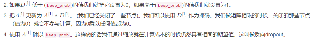
keep_prob - The probability of randomly deleting nodes is set to a value less than 1 when regularization is turned on.
return
parameters - Parameters after learning
"""
grads = {}
costs = []
m = X.shape[1]
layers_dims = [X.shape[0], 20, 3, 1]
# Initialization parameters
parameters = reg_utils.initialize_parameters(layers_dims)
# Start learning
for i in range(0, num_iterations):
# Forward propagation
##Delete nodes randomly
if keep_prob == 1:
###Do not randomly delete nodes
a3, cache = reg_utils.forward_propagation(X, parameters)
elif keep_prob < 1:
###Randomly delete nodes
a3, cache = forward_propagation_with_dropout(X, parameters, keep_prob)
else:
print("keep_prob Parameter error! Program exit.")
exit
# Calculate cost
## Whether to use two norm
if lambd == 0:
###L2 regularization is not used
cost = reg_utils.compute_cost(a3, Y)
else:
###Using L2 regularization
cost = compute_cost_with_regularization(a3, Y, parameters, lambd)
# Back propagation
##L2 regularization and random deletion of nodes can be used at the same time, but not in this experiment.
assert (lambd == 0 or keep_prob == 1)
##Usage of two parameters
if (lambd == 0 and keep_prob == 1):
### Do not use L2 regularization and do not use random deletion of nodes
grads = reg_utils.backward_propagation(X, Y, cache)
elif lambd != 0:
### L2 regularization is used instead of randomly deleting nodes
grads = backward_propagation_with_regularization(X, Y, cache, lambd)
elif keep_prob < 1:
### Randomly delete nodes without L2 regularization
grads = backward_propagation_with_dropout(X, Y, cache, keep_prob)
# Update parameters
parameters = reg_utils.update_parameters(parameters, grads, learning_rate)
# Record and print costs
if i % 1000 == 0:
## Record cost
costs.append(cost)
if (print_cost and i % 10000 == 0):
# Print cost
print("The first" + str(i) + "For the second iteration, the cost value is:" + str(cost))
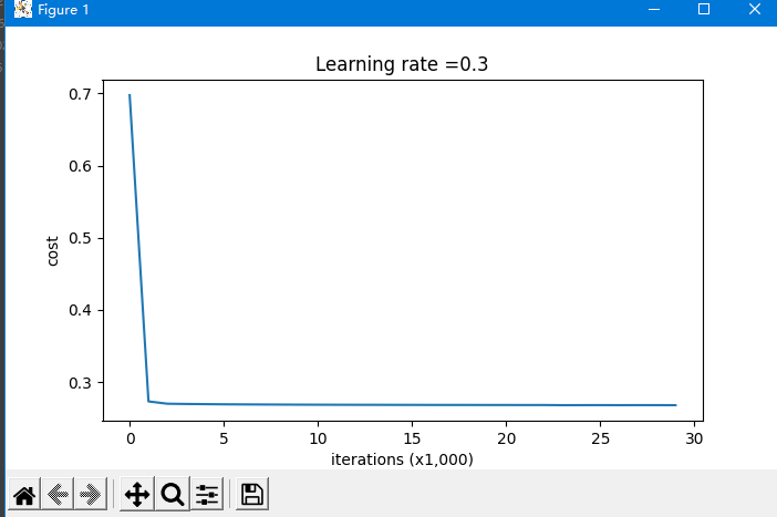
# Whether to draw cost curve
if is_plot:
plt.plot(costs)
plt.ylabel('cost')
plt.xlabel('iterations (x1,000)')
plt.title("Learning rate =" + str(learning_rate))
plt.show()
# Return learned parameters
return parameters
# Training without regularization and showing accuracy
parameters = model(train_X, train_Y,is_plot=True)
print("Training set:")
predictions_train = reg_utils.predict(train_X, train_Y, parameters)
print("Test set:")
predictions_test = reg_utils.predict(test_X, test_Y, parameters)
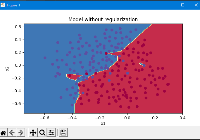
# Prediction results of data
plt.title("Model without regularization")
axes = plt.gca()
axes.set_xlim([-0.75,0.40])
axes.set_ylim([-0.75,0.65])
reg_utils.plot_decision_boundary(lambda x: reg_utils.predict_dec(parameters, x.T), train_X, train_Y)
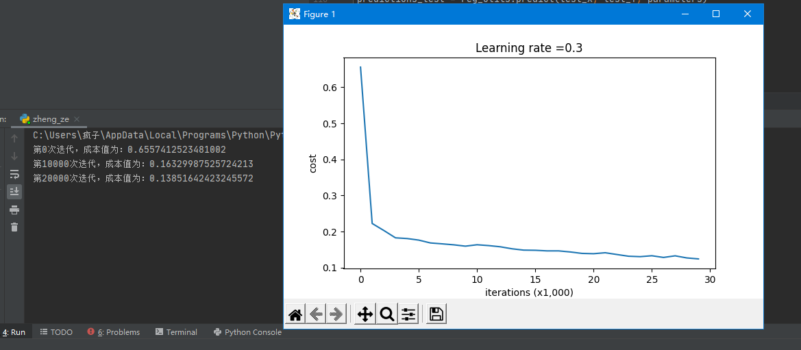
It can be seen that the training accuracy is 94.8%, while the test accuracy is 91.5%
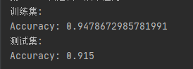
As can be seen from the figure below, the non regularized model obviously over fitted the training set and fitted some noise points!
Using L2 regularization
The loss function using L2 regularization needs to be modified, as shown below
J
just
be
turn
=
−
1
m
∑
i
=
1
m
(
y
(
i
)
log
(
a
[
L
]
(
i
)
)
+
(
1
−
y
(
i
)
)
log
(
1
−
a
[
L
]
(
i
)
)
)
⏟
cross-entropy cost
+
1
m
λ
2
∑
l
∑
k
∑
j
W
k
,
j
[
l
]
2
⏟
L2 Regularization cost
(2)
In the face of the J {thatis the beginning of the J {}}}}}}} thefollowing from the beginning of the first of the following of the J {{{{{{{{}} = = = = completingthe beginning of the first of the J of the J of the J of the j} = = = \ small \ underbattle {- \ frac{\ frac{\ underbattle{\ frac {{{1 {{{{{{{{{{{{{{{{}} \\} \ full full full} \ amount amount {{\\\\k \ sum \ limits_j w {K, J} ^ {[l] 2} \ text {L2 regularization cost} \ tag{2}
J regularization = cross entropy cost
−m1i=1∑m(y(i)log(a[L](i))+(1−y(i))log(1−a[L](i)))+L2 Regularization cost
m12λl∑k∑j∑Wk,j[l]2(2)
calculation
∑
k
∑
j
W
k
,
j
[
l
]
2
\sum\limits_k\sum\limits_j W_{k,j}^{[l]2}
The code of k Σ J Σ Wk,j[l]2 is np.sum(np.square(Wl)).
Note: you must
W
[
1
]
W^{[1]}
W[1],
W
[
2
]
W^{[2]}
W[2],
W
[
3
]
W^{[3]}
W[3] do this, then add the three items and multiply by
1
m
λ
2
\frac{1}{m}\frac{\lambda}{2}
m12λ.
# Cost function calculation of L2 regularization
def compute_cost_with_regularization(A3, Y, parameters, lambd):
    """
    Implementation of formula 2 L2 Regularization calculation cost

    Parameters:
        A3 - The dimension of the output result of forward propagation is (number of output nodes, training/Number of tests)
        Y - The label vector corresponds to the data one by one, and the dimension is(Number of output nodes, training/Number of tests)
        parameters - Dictionary containing parameters after model learning
    return:
        cost - The value of the regularization loss calculated using equation 2

    """
    m = Y.shape[1]
    W1 = parameters["W1"]
    W2 = parameters["W2"]
    W3 = parameters["W3"]

    cross_entropy_cost = reg_utils.compute_cost(A3, Y)

    L2_regularization_cost = lambd * (np.sum(np.square(W1)) + np.sum(np.square(W2)) + np.sum(np.square(W3))) / (2 * m)

    cost = cross_entropy_cost + L2_regularization_cost

    return cost
Because the cost function J is changed, the backward propagation also needs to be redefined. The code is as follows
Gradient calculation formula of regularization part
d
d
W
(
1
2
λ
m
W
2
)
=
λ
m
W
\frac{d}{dW} ( \frac{1}{2}\frac{\lambda}{m} W^2) = \frac{\lambda}{m} W
dWd(21mλW2)=mλW
def backward_propagation_with_regularization(X, Y, cache, lambd):
    """
    Implementation we added L2 Backward propagation of regularized model.

    Parameters:
        X - Enter a dataset with dimension (enter the number of nodes and the number in the dataset)
        Y - Label, dimension is (number of output nodes, number in dataset)
        cache - come from forward_propagation()of cache output
        lambda - regularization Super parameter, real number

    return:
        gradients - A dictionary containing gradients for each parameter, activation value, and pre activation value variable
    """

    m = X.shape[1]

    (Z1, A1, W1, b1, Z2, A2, W2, b2, Z3, A3, W3, b3) = cache

    dZ3 = A3 - Y

    dW3 = (1 / m) * np.dot(dZ3, A2.T) + ((lambd * W3) / m)
    db3 = (1 / m) * np.sum(dZ3, axis=1, keepdims=True)

    dA2 = np.dot(W3.T, dZ3)
    dZ2 = np.multiply(dA2, np.int64(A2 > 0))
    dW2 = (1 / m) * np.dot(dZ2, A1.T) + ((lambd * W2) / m)
    db2 = (1 / m) * np.sum(dZ2, axis=1, keepdims=True)

    dA1 = np.dot(W2.T, dZ2)
    dZ1 = np.multiply(dA1, np.int64(A1 > 0))
    dW1 = (1 / m) * np.dot(dZ1, X.T) + ((lambd * W1) / m)
    db1 = (1 / m) * np.sum(dZ1, axis=1, keepdims=True)

    gradients = {"dZ3": dZ3, "dW3": dW3, "db3": db3, "dA2": dA2,
                 "dZ2": dZ2, "dW2": dW2, "db2": db2, "dA1": dA1,
                 "dZ1": dZ1, "dW1": dW1, "db1": db1}

    return gradients
Now we use L2 regularization to train the model and output the accuracy, cost function, Image J, and prediction classification results.
import numpy as np
import matplotlib.pyplot as plt
import reg_utils
from reg_utils import sigmoid, relu, plot_decision_boundary, initialize_parameters, load_2D_dataset, predict_dec
from reg_utils import compute_cost, predict, forward_propagation, backward_propagation, update_parameters
import sklearn
import sklearn.datasets
import scipy.io
from testCases import *
plt.rcParams['figure.figsize'] = (7.0, 4.0) # set default size of plots
plt.rcParams['image.interpolation'] = 'nearest'
plt.rcParams['image.cmap'] = 'gray'
train_X, train_Y, test_X, test_Y = load_2D_dataset()
plt.show()
# Define our model
def model(X, Y, learning_rate=0.3, num_iterations=30000, print_cost=True, is_plot=True, lambd=0, keep_prob=1):
"""
Implement a three-layer neural network: LINEAR ->RELU -> LINEAR -> RELU -> LINEAR -> SIGMOID
Parameters:
X - The dimension of the entered data is(2, To train/Number of tests)
Y - Label, [0](blue) | 1(gules)],Dimension is(1,This corresponds to the label of the input data)
learning_rate - Learning rate
num_iterations - Number of iterations
print_cost - Whether to print the cost value. Print once every 10000 iterations, but record one cost value every 1000 iterations
is_polt - Whether to draw the curve of gradient descent
lambd - Regularized hyperparameters, real numbers, will lambd If the input is set to a non-zero value, regularization is enabled; otherwise, regularization is turned off
We use“ lambd"Not“ lambda",Because“ lambda"yes Python Reserved keywords in
keep_prob - The probability of randomly deleting nodes is set to a value less than 1 when regularization is turned on.
return
parameters - Parameters after learning
"""
grads = {}
costs = []
m = X.shape[1]
layers_dims = [X.shape[0], 20, 3, 1]
# Initialization parameters
parameters = reg_utils.initialize_parameters(layers_dims)
# Start learning
for i in range(0, num_iterations):
# Forward propagation
##Delete nodes randomly
if keep_prob == 1:
###Do not randomly delete nodes
a3, cache = reg_utils.forward_propagation(X, parameters)
elif keep_prob < 1:
###Randomly delete nodes
a3, cache = forward_propagation_with_dropout(X, parameters, keep_prob)
else:
print("keep_prob Parameter error! Program exit.")
exit
# Calculate cost
## Whether to use two norm
if lambd == 0:
###L2 regularization is not used
cost = reg_utils.compute_cost(a3, Y)
else:
###Using L2 regularization
cost = compute_cost_with_regularization(a3, Y, parameters, lambd)
# Back propagation
##L2 regularization and random deletion of nodes can be used at the same time, but not in this experiment.
assert (lambd == 0 or keep_prob == 1)
##Usage of two parameters
if (lambd == 0 and keep_prob == 1):
### Do not use L2 regularization and do not use random deletion of nodes
grads = reg_utils.backward_propagation(X, Y, cache)
elif lambd != 0:
### L2 regularization is used instead of randomly deleting nodes
grads = backward_propagation_with_regularization(X, Y, cache, lambd)
elif keep_prob < 1:
### Randomly delete nodes without L2 regularization
grads = backward_propagation_with_dropout(X, Y, cache, keep_prob)
# Update parameters
parameters = reg_utils.update_parameters(parameters, grads, learning_rate)
# Record and print costs
if i % 1000 == 0:
## Record cost
costs.append(cost)
if (print_cost and i % 10000 == 0):
# Print cost
print("The first" + str(i) + "For the second iteration, the cost value is:" + str(cost))
# Whether to draw cost curve
if is_plot:
plt.plot(costs)
plt.ylabel('cost')
plt.xlabel('iterations (x1,000)')
plt.title("Learning rate =" + str(learning_rate))
plt.show()
# Return learned parameters
return parameters
# Training without regularization and showing accuracy
# parameters = model(train_X, train_Y,is_plot=True)
# print("training set:")
# predictions_train = reg_utils.predict(train_X, train_Y, parameters)
# print("test set:")
# predictions_test = reg_utils.predict(test_X, test_Y, parameters)
# Prediction results of data
# plt.title("Model without regularization")
# axes = plt.gca()
# axes.set_xlim([-0.75,0.40])
# axes.set_ylim([-0.75,0.65])
# reg_utils.plot_decision_boundary(lambda x: reg_utils.predict_dec(parameters, x.T), train_X, train_Y)
# Cost function calculation of L2 regularization
def compute_cost_with_regularization(A3, Y, parameters, lambd):
"""
Implementation of formula 2 L2 Regularization calculation cost
Parameters:
A3 - The dimension of the output result of forward propagation is (number of output nodes, training/Number of tests)
Y - The label vector corresponds to the data one by one, and the dimension is(Number of output nodes, training/Number of tests)
parameters - Dictionary containing parameters after model learning
return:
cost - The value of the regularization loss calculated using equation 2
"""
m = Y.shape[1]
W1 = parameters["W1"]
W2 = parameters["W2"]
W3 = parameters["W3"]
cross_entropy_cost = reg_utils.compute_cost(A3, Y)
L2_regularization_cost = lambd * (np.sum(np.square(W1)) + np.sum(np.square(W2)) + np.sum(np.square(W3))) / (2 * m)
cost = cross_entropy_cost + L2_regularization_cost
return cost
# Of course, because the cost function is changed, we must also change the back-propagation function, and all gradients must be calculated according to the new cost value.
def backward_propagation_with_regularization(X, Y, cache, lambd):
"""
Implementation we added L2 Backward propagation of regularized model.
Parameters:
X - Enter a dataset with dimension (enter the number of nodes and the number in the dataset)
Y - Label, dimension is (number of output nodes, number in dataset)
cache - come from forward_propagation()of cache output
lambda - regularization Super parameter, real number
return:
gradients - A dictionary containing gradients for each parameter, activation value, and pre activation value variable
"""
m = X.shape[1]
(Z1, A1, W1, b1, Z2, A2, W2, b2, Z3, A3, W3, b3) = cache
dZ3 = A3 - Y
dW3 = (1 / m) * np.dot(dZ3, A2.T) + ((lambd * W3) / m)
db3 = (1 / m) * np.sum(dZ3, axis=1, keepdims=True)
dA2 = np.dot(W3.T, dZ3)
dZ2 = np.multiply(dA2, np.int64(A2 > 0))
dW2 = (1 / m) * np.dot(dZ2, A1.T) + ((lambd * W2) / m)
db2 = (1 / m) * np.sum(dZ2, axis=1, keepdims=True)
dA1 = np.dot(W2.T, dZ2)
dZ1 = np.multiply(dA1, np.int64(A1 > 0))
dW1 = (1 / m) * np.dot(dZ1, X.T) + ((lambd * W1) / m)
db1 = (1 / m) * np.sum(dZ1, axis=1, keepdims=True)
gradients = {"dZ3": dZ3, "dW3": dW3, "db3": db3, "dA2": dA2,
"dZ2": dZ2, "dW2": dW2, "db2": db2, "dA1": dA1,
"dZ1": dZ1, "dW1": dW1, "db1": db1}
return gradients
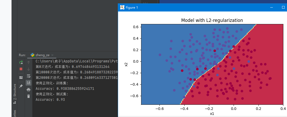
# Model training using L2 regularization
parameters = model(train_X, train_Y, lambd=0.7,is_plot=True)
# Output accuracy
print("Using regularization, the training set:")
predictions_train = reg_utils.predict(train_X, train_Y, parameters)
print("Using regularization, test set:")
predictions_test = reg_utils.predict(test_X, test_Y, parameters)
#View the classification results of the dataset
plt.title("Model with L2-regularization")
axes = plt.gca()
axes.set_xlim([-0.75,0.40])
axes.set_ylim([-0.75,0.65])
reg_utils.plot_decision_boundary(lambda x: reg_utils.predict_dec(parameters, x.T), train_X, train_Y)
As can be seen from the results in the figure below, our accuracy has been improved to 93.5%
Note: lambd in the code means λ, Is a hyperparameter, L2 regularization is to make the boundary smoother if λ Too large, it may be too smooth. Impact of L2 regularization: regularization conditions will be added to the loss function. In the gradient of the weight matrix, the weight will eventually become smaller ("weight attenuation"), and the weight will be pushed to a smaller value.
Random deactivation using Dropout
Dropout is a regularization technique widely used for deep learning. It turns off some neurons at random in each iteration. In each iteration, you turn off some neurons in a layer with probability keep prop. Both forward and back propagation of closed neurons to iteration are not conducive to training. The principle of execution is as follows:

Create a dropout.py file. Under the same project folder, import relevant libraries, load data and define neural network model.
import numpy as np
import matplotlib.pyplot as plt
import reg_utils
from reg_utils import sigmoid, relu, plot_decision_boundary, initialize_parameters, load_2D_dataset, predict_dec
from reg_utils import compute_cost, predict, forward_propagation, backward_propagation, update_parameters
import sklearn
import sklearn.datasets
import scipy.io
from testCases import *


plt.rcParams['figure.figsize'] = (7.0, 4.0) # set default size of plots
plt.rcParams['image.interpolation'] = 'nearest'
plt.rcParams['image.cmap'] = 'gray'

train_X, train_Y, test_X, test_Y = load_2D_dataset()
plt.show()

# Define our model
def model(X, Y, learning_rate=0.3, num_iterations=30000, print_cost=True, is_plot=True, lambd=0, keep_prob=1):
    """
    Implement a three-layer neural network: LINEAR ->RELU -> LINEAR -> RELU -> LINEAR -> SIGMOID

    Parameters:
        X - The dimension of the entered data is(2, To train/Number of tests)
        Y - Label, [0](blue) | 1(gules)],Dimension is(1,This corresponds to the label of the input data)
        learning_rate - Learning rate
        num_iterations - Number of iterations
        print_cost - Whether to print the cost value. Print once every 10000 iterations, but record one cost value every 1000 iterations
        is_polt - Whether to draw the curve of gradient descent
        lambd - Regularized hyperparameters, real numbers, will lambd If the input is set to a non-zero value, regularization is enabled; otherwise, regularization is turned off
        We use“ lambd"Not“ lambda",Because“ lambda"yes Python Reserved keywords in
        keep_prob - The probability of randomly deleting nodes is set to a value less than 1 when regularization is turned on.
    return
        parameters - Parameters after learning
    """
    grads = {}
    costs = []
    m = X.shape[1]
    layers_dims = [X.shape[0], 20, 3, 1]

    # Initialization parameters
    parameters = reg_utils.initialize_parameters(layers_dims)

    # Start learning
    for i in range(0, num_iterations):
        # Forward propagation
        ##Delete nodes randomly
        if keep_prob == 1:
            ###Do not randomly delete nodes
            a3, cache = reg_utils.forward_propagation(X, parameters)
        elif keep_prob < 1:
            ###Randomly delete nodes
            a3, cache = forward_propagation_with_dropout(X, parameters, keep_prob)
        else:
            print("keep_prob Parameter error! Program exit.")
            exit

        # Calculate cost
        ## Whether to use two norm
        if lambd == 0:
            ###L2 regularization is not used
            cost = reg_utils.compute_cost(a3, Y)
        else:
            ###Using L2 regularization
            cost = compute_cost_with_regularization(a3, Y, parameters, lambd)

        # Back propagation
        ##L2 regularization and random deletion of nodes can be used at the same time, but not in this experiment.
        assert (lambd == 0 or keep_prob == 1)

        ##Usage of two parameters
        if (lambd == 0 and keep_prob == 1):
            ### Do not use L2 regularization and do not use random deletion of nodes
            grads = reg_utils.backward_propagation(X, Y, cache)
        elif lambd != 0:
            ### L2 regularization is used instead of randomly deleting nodes
            grads = backward_propagation_with_regularization(X, Y, cache, lambd)
        elif keep_prob < 1:
            ### Randomly delete nodes without L2 regularization
            grads = backward_propagation_with_dropout(X, Y, cache, keep_prob)

        # Update parameters
        parameters = reg_utils.update_parameters(parameters, grads, learning_rate)

        # Record and print costs
        if i % 1000 == 0:
            ## Record cost
            costs.append(cost)
            if (print_cost and i % 10000 == 0):
                # Print cost
                print("The first" + str(i) + "For the second iteration, the cost value is:" + str(cost))

    # Whether to draw cost curve
    if is_plot:
        plt.plot(costs)
        plt.ylabel('cost')
        plt.xlabel('iterations (x1,000)')
        plt.title("Learning rate =" + str(learning_rate))
        plt.show()

    # Return learned parameters
    return parameters
# Define dropout random deactivation forward propagation
def forward_propagation_with_dropout(X, parameters, keep_prob=0.5):
    """
    Forward propagation with randomly discarded nodes is realized.
    LINEAR -> RELU + DROPOUT -> LINEAR -> RELU + DROPOUT -> LINEAR -> SIGMOID.

    Parameters:
        X  - Input dataset, dimension is (2, number of examples)
        parameters - Include parameters“ W1","b1","W2","b2","W3","b3"of python Dictionaries:
            W1  - Weight matrix with dimension of (20),2)
            b1  - Bias, dimension (20),1)
            W2  - Weight matrix with dimension (3),20)
            b2  - Bias, dimension (3),1)
            W3  - Weight matrix with dimension (1),3)
            b3  - Bias, dimension (1),1)
        keep_prob  - Probability of random deletion, real number
    return:
        A3  - The last activation value, dimension (1),1),Forward propagating output
        cache - Some tuples of values used to calculate back propagation are stored
    """
    np.random.seed(1)

    W1 = parameters["W1"]
    b1 = parameters["b1"]
    W2 = parameters["W2"]
    b2 = parameters["b2"]
    W3 = parameters["W3"]
    b3 = parameters["b3"]

    # LINEAR -> RELU -> LINEAR -> RELU -> LINEAR -> SIGMOID
    Z1 = np.dot(W1, X) + b1
    A1 = reg_utils.relu(Z1)

    # The following steps 1-4 correspond to the above steps 1-4.
    D1 = np.random.rand(A1.shape[0], A1.shape[1])  # Step 1: initialize the matrix D1 = np.random.rand(...,...)
    D1 = D1 < keep_prob  # Step 2: convert the value of D1 to 0 or 1 (use keep_prob as the threshold)
    A1 = A1 * D1  # Step 3: discard some nodes of A1 (change its value to 0 or False)
    A1 = A1 / keep_prob  # Step 4: scale the value of the UN discarded node (not 0)
    """
    #If you don't understand, just run the following code.
    import numpy as np
    np.random.seed(1)
    A1 = np.random.randn(1,3)

    D1 = np.random.rand(A1.shape[0],A1.shape[1])
    keep_prob=0.5
    D1 = D1 < keep_prob
    print(D1)

    A1 = 0.01
    A1 = A1 * D1
    A1 = A1 / keep_prob
    print(A1)
    """

    Z2 = np.dot(W2, A1) + b2
    A2 = reg_utils.relu(Z2)

    # The following steps 1-4 correspond to the above steps 1-4.
    D2 = np.random.rand(A2.shape[0], A2.shape[1])  # Step 1: initialize matrix D2 = np.random.rand(...,...)
    D2 = D2 < keep_prob  # Step 2: convert the value of D2 to 0 or 1 (use keep_prob as the threshold)
    A2 = A2 * D2  # Step 3: discard some nodes of A1 (change its value to 0 or False)
    A2 = A2 / keep_prob  # Step 4: scale the value of the UN discarded node (not 0)

    Z3 = np.dot(W3, A2) + b3
    A3 = reg_utils.sigmoid(Z3)

    cache = (Z1, D1, A1, W1, b1, Z2, D2, A2, W2, b2, Z3, A3, W3, b3)

    return A3, cache
# The corresponding backward propagation function is changed
def backward_propagation_with_dropout(X, Y, cache, keep_prob):
    """
    Implement the backward propagation of our randomly deleted model.
    Parameters:
        X  - Input dataset, dimension is (2, number of examples)
        Y  - Label, dimension is (number of output nodes, number of samples)
        cache - come from forward_propagation_with_dropout()of cache output
        keep_prob  - Probability of random deletion, real number

    return:
        gradients - A dictionary of gradient values for each parameter, activation value, and pre activation variable
    """
    m = X.shape[1]
    (Z1, D1, A1, W1, b1, Z2, D2, A2, W2, b2, Z3, A3, W3, b3) = cache

    dZ3 = A3 - Y
    dW3 = (1 / m) * np.dot(dZ3, A2.T)
    db3 = 1. / m * np.sum(dZ3, axis=1, keepdims=True)
    dA2 = np.dot(W3.T, dZ3)

    dA2 = dA2 * D2  # Step 1: use the same nodes during forward propagation and discard those closed nodes (because any number multiplied by 0 or False is 0 or False)
    dA2 = dA2 / keep_prob  # Step 2: scale the value of the UN discarded node (not 0)

    dZ2 = np.multiply(dA2, np.int64(A2 > 0))
    dW2 = 1. / m * np.dot(dZ2, A1.T)
    db2 = 1. / m * np.sum(dZ2, axis=1, keepdims=True)

    dA1 = np.dot(W2.T, dZ2)

    dA1 = dA1 * D1  # Step 1: use the same nodes during forward propagation and discard those closed nodes (because any number multiplied by 0 or False is 0 or False)
    dA1 = dA1 / keep_prob  # Step 2: scale the value of the UN discarded node (not 0)

    dZ1 = np.multiply(dA1, np.int64(A1 > 0))
    dW1 = 1. / m * np.dot(dZ1, X.T)
    db1 = 1. / m * np.sum(dZ1, axis=1, keepdims=True)

    gradients = {"dZ3": dZ3, "dW3": dW3, "db3": db3, "dA2": dA2,
                 "dZ2": dZ2, "dW2": dW2, "db2": db2, "dA1": dA1,
                 "dZ1": dZ1, "dW1": dW1, "db1": db1}

    return gradients
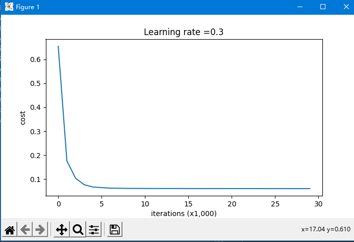
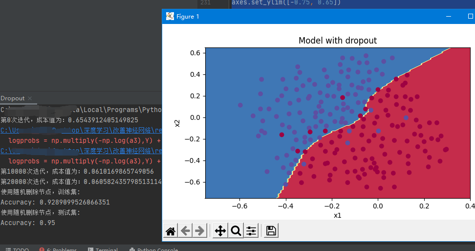
Next, we use dropout regularization to train the model, and show the accuracy, cost function J and final prediction classification
# The training model uses dropou regularization, with a 14 percent (0.14) probability of losing some neural units each time
parameters = model(train_X, train_Y, keep_prob=0.86, learning_rate=0.3,is_plot=True)

print("Use to randomly delete nodes, training sets:")
predictions_train = reg_utils.predict(train_X, train_Y, parameters)
print("Test set using randomly deleted nodes:")
reg_utils.predictions_test = reg_utils.predict(test_X, test_Y, parameters)

# View forecast classification
plt.title("Model with dropout")
axes = plt.gca()
axes.set_xlim([-0.75, 0.40])
axes.set_ylim([-0.75, 0.65])
reg_utils.plot_decision_boundary(lambda x: reg_utils.predict_dec(parameters, x.T), train_X, train_Y)
be careful:
- dropout is a regularization technique.
- Use dropout only during training and not during testing.
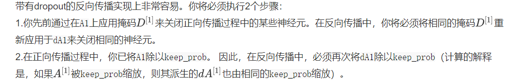
- dropout is applied during both forward and reverse propagation.
Regularization complete code
import numpy as np
import matplotlib.pyplot as plt
import reg_utils
from reg_utils import sigmoid, relu, plot_decision_boundary, initialize_parameters, load_2D_dataset, predict_dec
from reg_utils import compute_cost, predict, forward_propagation, backward_propagation, update_parameters
import sklearn
import sklearn.datasets
import scipy.io
from testCases import *


plt.rcParams['figure.figsize'] = (7.0, 4.0) # set default size of plots
plt.rcParams['image.interpolation'] = 'nearest'
plt.rcParams['image.cmap'] = 'gray'

train_X, train_Y, test_X, test_Y = load_2D_dataset()
plt.show()

# Define our model
def model(X, Y, learning_rate=0.3, num_iterations=30000, print_cost=True, is_plot=True, lambd=0, keep_prob=1):
    """
    Implement a three-layer neural network: LINEAR ->RELU -> LINEAR -> RELU -> LINEAR -> SIGMOID

    Parameters:
        X - The dimension of the entered data is(2, To train/Number of tests)
        Y - Label, [0](blue) | 1(gules)],Dimension is(1,This corresponds to the label of the input data)
        learning_rate - Learning rate
        num_iterations - Number of iterations
        print_cost - Whether to print the cost value. Print once every 10000 iterations, but record one cost value every 1000 iterations
        is_polt - Whether to draw the curve of gradient descent
        lambd - Regularized hyperparameters, real numbers, will lambd If the input is set to a non-zero value, regularization is enabled; otherwise, regularization is turned off
        We use“ lambd"Not“ lambda",Because“ lambda"yes Python Reserved keywords in
        keep_prob - The probability of randomly deleting nodes is set to a value less than 1 when regularization is turned on.
    return
        parameters - Parameters after learning
    """
    grads = {}
    costs = []
    m = X.shape[1]
    layers_dims = [X.shape[0], 20, 3, 1]

    # Initialization parameters
    parameters = reg_utils.initialize_parameters(layers_dims)

    # Start learning
    for i in range(0, num_iterations):
        # Forward propagation
        ##Delete nodes randomly
        if keep_prob == 1:
            ###Do not randomly delete nodes
            a3, cache = reg_utils.forward_propagation(X, parameters)
        elif keep_prob < 1:
            ###Randomly delete nodes
            a3, cache = forward_propagation_with_dropout(X, parameters, keep_prob)
        else:
            print("keep_prob Parameter error! Program exit.")
            exit

        # Calculate cost
        ## Whether to use two norm
        if lambd == 0:
            ###L2 regularization is not used
            cost = reg_utils.compute_cost(a3, Y)
        else:
            ###Using L2 regularization
            cost = compute_cost_with_regularization(a3, Y, parameters, lambd)

        # Back propagation
        ##L2 regularization and random deletion of nodes can be used at the same time, but not in this experiment.
        assert (lambd == 0 or keep_prob == 1)

        ##Usage of two parameters
        if (lambd == 0 and keep_prob == 1):
            ### Do not use L2 regularization and do not use random deletion of nodes
            grads = reg_utils.backward_propagation(X, Y, cache)
        elif lambd != 0:
            ### L2 regularization is used instead of randomly deleting nodes
            grads = backward_propagation_with_regularization(X, Y, cache, lambd)
        elif keep_prob < 1:
            ### Randomly delete nodes without L2 regularization
            grads = backward_propagation_with_dropout(X, Y, cache, keep_prob)

        # Update parameters
        parameters = reg_utils.update_parameters(parameters, grads, learning_rate)

        # Record and print costs
        if i % 1000 == 0:
            ## Record cost
            costs.append(cost)
            if (print_cost and i % 10000 == 0):
                # Print cost
                print("The first" + str(i) + "For the second iteration, the cost value is:" + str(cost))

    # Whether to draw cost curve
    if is_plot:
        plt.plot(costs)
        plt.ylabel('cost')
        plt.xlabel('iterations (x1,000)')
        plt.title("Learning rate =" + str(learning_rate))
        plt.show()

    # Return learned parameters
    return parameters

# Training without regularization and showing accuracy
# parameters = model(train_X, train_Y,is_plot=True)
# print("training set:")
# predictions_train = reg_utils.predict(train_X, train_Y, parameters)
# print("test set:")
# predictions_test = reg_utils.predict(test_X, test_Y, parameters)

# Prediction results of data
# plt.title("Model without regularization")
# axes = plt.gca()
# axes.set_xlim([-0.75,0.40])
# axes.set_ylim([-0.75,0.65])
# reg_utils.plot_decision_boundary(lambda x: reg_utils.predict_dec(parameters, x.T), train_X, train_Y)

# Cost function calculation of L2 regularization
def compute_cost_with_regularization(A3, Y, parameters, lambd):
    """
    Implementation of formula 2 L2 Regularization calculation cost

    Parameters:
        A3 - The dimension of the output result of forward propagation is (number of output nodes, training/Number of tests)
        Y - The label vector corresponds to the data one by one, and the dimension is(Number of output nodes, training/Number of tests)
        parameters - Dictionary containing parameters after model learning
    return:
        cost - The value of the regularization loss calculated using equation 2

    """
    m = Y.shape[1]
    W1 = parameters["W1"]
    W2 = parameters["W2"]
    W3 = parameters["W3"]

    cross_entropy_cost = reg_utils.compute_cost(A3, Y)

    L2_regularization_cost = lambd * (np.sum(np.square(W1)) + np.sum(np.square(W2)) + np.sum(np.square(W3))) / (2 * m)

    cost = cross_entropy_cost + L2_regularization_cost

    return cost


# Of course, because the cost function is changed, we must also change the back-propagation function, and all gradients must be calculated according to the new cost value.
def backward_propagation_with_regularization(X, Y, cache, lambd):
    """
    Implementation we added L2 Backward propagation of regularized model.

    Parameters:
        X - Enter a dataset with dimension (enter the number of nodes and the number in the dataset)
        Y - Label, dimension is (number of output nodes, number in dataset)
        cache - come from forward_propagation()of cache output
        lambda - regularization Super parameter, real number

    return:
        gradients - A dictionary containing gradients for each parameter, activation value, and pre activation value variable
    """

    m = X.shape[1]

    (Z1, A1, W1, b1, Z2, A2, W2, b2, Z3, A3, W3, b3) = cache

    dZ3 = A3 - Y

    dW3 = (1 / m) * np.dot(dZ3, A2.T) + ((lambd * W3) / m)
    db3 = (1 / m) * np.sum(dZ3, axis=1, keepdims=True)

    dA2 = np.dot(W3.T, dZ3)
    dZ2 = np.multiply(dA2, np.int64(A2 > 0))
    dW2 = (1 / m) * np.dot(dZ2, A1.T) + ((lambd * W2) / m)
    db2 = (1 / m) * np.sum(dZ2, axis=1, keepdims=True)

    dA1 = np.dot(W2.T, dZ2)
    dZ1 = np.multiply(dA1, np.int64(A1 > 0))
    dW1 = (1 / m) * np.dot(dZ1, X.T) + ((lambd * W1) / m)
    db1 = (1 / m) * np.sum(dZ1, axis=1, keepdims=True)

    gradients = {"dZ3": dZ3, "dW3": dW3, "db3": db3, "dA2": dA2,
                 "dZ2": dZ2, "dW2": dW2, "db2": db2, "dA1": dA1,
                 "dZ1": dZ1, "dW1": dW1, "db1": db1}

    return gradients

# Model training using L2 regularization
parameters = model(train_X, train_Y, lambd=0.7,is_plot=True)

# Output accuracy
print("Using regularization, the training set:")
predictions_train = reg_utils.predict(train_X, train_Y, parameters)
print("Using regularization, test set:")
predictions_test = reg_utils.predict(test_X, test_Y, parameters)

#View the classification results of the dataset
plt.title("Model with L2-regularization")
axes = plt.gca()
axes.set_xlim([-0.75,0.40])
axes.set_ylim([-0.75,0.65])
reg_utils.plot_decision_boundary(lambda x: reg_utils.predict_dec(parameters, x.T), train_X, train_Y)
Random deactivation complete code
import numpy as np
import matplotlib.pyplot as plt
import reg_utils
from reg_utils import sigmoid, relu, plot_decision_boundary, initialize_parameters, load_2D_dataset, predict_dec
from reg_utils import compute_cost, predict, forward_propagation, backward_propagation, update_parameters
import sklearn
import sklearn.datasets
import scipy.io
from testCases import *


plt.rcParams['figure.figsize'] = (7.0, 4.0) # set default size of plots
plt.rcParams['image.interpolation'] = 'nearest'
plt.rcParams['image.cmap'] = 'gray'

train_X, train_Y, test_X, test_Y = load_2D_dataset()
plt.show()

# Define our model
def model(X, Y, learning_rate=0.3, num_iterations=30000, print_cost=True, is_plot=True, lambd=0, keep_prob=1):
    """
    Implement a three-layer neural network: LINEAR ->RELU -> LINEAR -> RELU -> LINEAR -> SIGMOID

    Parameters:
        X - The dimension of the entered data is(2, To train/Number of tests)
        Y - Label, [0](blue) | 1(gules)],Dimension is(1,This corresponds to the label of the input data)
        learning_rate - Learning rate
        num_iterations - Number of iterations
        print_cost - Whether to print the cost value. Print once every 10000 iterations, but record one cost value every 1000 iterations
        is_polt - Whether to draw the curve of gradient descent
        lambd - Regularized hyperparameters, real numbers, will lambd If the input is set to a non-zero value, regularization is enabled; otherwise, regularization is turned off
        We use“ lambd"Not“ lambda",Because“ lambda"yes Python Reserved keywords in
        keep_prob - The probability of randomly deleting nodes is set to a value less than 1 when regularization is turned on.
    return
        parameters - Parameters after learning
    """
    grads = {}
    costs = []
    m = X.shape[1]
    layers_dims = [X.shape[0], 20, 3, 1]

    # Initialization parameters
    parameters = reg_utils.initialize_parameters(layers_dims)

    # Start learning
    for i in range(0, num_iterations):
        # Forward propagation
        ##Delete nodes randomly
        if keep_prob == 1:
            ###Do not randomly delete nodes
            a3, cache = reg_utils.forward_propagation(X, parameters)
        elif keep_prob < 1:
            ###Randomly delete nodes
            a3, cache = forward_propagation_with_dropout(X, parameters, keep_prob)
        else:
            print("keep_prob Parameter error! Program exit.")
            exit

        # Calculate cost
        ## Whether to use two norm
        if lambd == 0:
            ###L2 regularization is not used
            cost = reg_utils.compute_cost(a3, Y)
        else:
            ###Using L2 regularization
            cost = compute_cost_with_regularization(a3, Y, parameters, lambd)

        # Back propagation
        ##L2 regularization and random deletion of nodes can be used at the same time, but not in this experiment.
        assert (lambd == 0 or keep_prob == 1)

        ##Usage of two parameters
        if (lambd == 0 and keep_prob == 1):
            ### Do not use L2 regularization and do not use random deletion of nodes
            grads = reg_utils.backward_propagation(X, Y, cache)
        elif lambd != 0:
            ### L2 regularization is used instead of randomly deleting nodes
            grads = backward_propagation_with_regularization(X, Y, cache, lambd)
        elif keep_prob < 1:
            ### Randomly delete nodes without L2 regularization
            grads = backward_propagation_with_dropout(X, Y, cache, keep_prob)

        # Update parameters
        parameters = reg_utils.update_parameters(parameters, grads, learning_rate)

        # Record and print costs
        if i % 1000 == 0:
            ## Record cost
            costs.append(cost)
            if (print_cost and i % 10000 == 0):
                # Print cost
                print("The first" + str(i) + "For the second iteration, the cost value is:" + str(cost))

    # Whether to draw cost curve
    if is_plot:
        plt.plot(costs)
        plt.ylabel('cost')
        plt.xlabel('iterations (x1,000)')
        plt.title("Learning rate =" + str(learning_rate))
        plt.show()

    # Return learned parameters
    return parameters

# Define dropout random deactivation forward propagation
def forward_propagation_with_dropout(X, parameters, keep_prob=0.5):
    """
    Forward propagation with randomly discarded nodes is realized.
    LINEAR -> RELU + DROPOUT -> LINEAR -> RELU + DROPOUT -> LINEAR -> SIGMOID.

    Parameters:
        X  - Input dataset, dimension is (2, number of examples)
        parameters - Include parameters“ W1","b1","W2","b2","W3","b3"of python Dictionaries:
            W1  - Weight matrix with dimension of (20),2)
            b1  - Bias, dimension (20),1)
            W2  - Weight matrix with dimension (3),20)
            b2  - Bias, dimension (3),1)
            W3  - Weight matrix with dimension (1),3)
            b3  - Bias, dimension (1),1)
        keep_prob  - Probability of random deletion, real number
    return:
        A3  - The last activation value, dimension (1),1),Forward propagating output
        cache - Some tuples of values used to calculate back propagation are stored
    """
    np.random.seed(1)

    W1 = parameters["W1"]
    b1 = parameters["b1"]
    W2 = parameters["W2"]
    b2 = parameters["b2"]
    W3 = parameters["W3"]
    b3 = parameters["b3"]

    # LINEAR -> RELU -> LINEAR -> RELU -> LINEAR -> SIGMOID
    Z1 = np.dot(W1, X) + b1
    A1 = reg_utils.relu(Z1)

    # The following steps 1-4 correspond to the above steps 1-4.
    D1 = np.random.rand(A1.shape[0], A1.shape[1])  # Step 1: initialize the matrix D1 = np.random.rand(...,...)
    D1 = D1 < keep_prob  # Step 2: convert the value of D1 to 0 or 1 (use keep_prob as the threshold)
    A1 = A1 * D1  # Step 3: discard some nodes of A1 (change its value to 0 or False)
    A1 = A1 / keep_prob  # Step 4: scale the value of the UN discarded node (not 0)
    """
    #If you don't understand, just run the following code.
    import numpy as np
    np.random.seed(1)
    A1 = np.random.randn(1,3)

    D1 = np.random.rand(A1.shape[0],A1.shape[1])
    keep_prob=0.5
    D1 = D1 < keep_prob
    print(D1)

    A1 = 0.01
    A1 = A1 * D1
    A1 = A1 / keep_prob
    print(A1)
    """

    Z2 = np.dot(W2, A1) + b2
    A2 = reg_utils.relu(Z2)

    # The following steps 1-4 correspond to the above steps 1-4.
    D2 = np.random.rand(A2.shape[0], A2.shape[1])  # Step 1: initialize matrix D2 = np.random.rand(...,...)
    D2 = D2 < keep_prob  # Step 2: convert the value of D2 to 0 or 1 (use keep_prob as the threshold)
    A2 = A2 * D2  # Step 3: discard some nodes of A1 (change its value to 0 or False)
    A2 = A2 / keep_prob  # Step 4: scale the value of the UN discarded node (not 0)

    Z3 = np.dot(W3, A2) + b3
    A3 = reg_utils.sigmoid(Z3)

    cache = (Z1, D1, A1, W1, b1, Z2, D2, A2, W2, b2, Z3, A3, W3, b3)

    return A3, cache

# The corresponding backward propagation function is changed
def backward_propagation_with_dropout(X, Y, cache, keep_prob):
    """
    Implement the backward propagation of our randomly deleted model.
    Parameters:
        X  - Input dataset, dimension is (2, number of examples)
        Y  - Label, dimension is (number of output nodes, number of samples)
        cache - come from forward_propagation_with_dropout()of cache output
        keep_prob  - Probability of random deletion, real number

    return:
        gradients - A dictionary of gradient values for each parameter, activation value, and pre activation variable
    """
    m = X.shape[1]
    (Z1, D1, A1, W1, b1, Z2, D2, A2, W2, b2, Z3, A3, W3, b3) = cache

    dZ3 = A3 - Y
    dW3 = (1 / m) * np.dot(dZ3, A2.T)
    db3 = 1. / m * np.sum(dZ3, axis=1, keepdims=True)
    dA2 = np.dot(W3.T, dZ3)

    dA2 = dA2 * D2  # Step 1: use the same nodes during forward propagation and discard those closed nodes (because any number multiplied by 0 or False is 0 or False)
    dA2 = dA2 / keep_prob  # Step 2: scale the value of the UN discarded node (not 0)

    dZ2 = np.multiply(dA2, np.int64(A2 > 0))
    dW2 = 1. / m * np.dot(dZ2, A1.T)
    db2 = 1. / m * np.sum(dZ2, axis=1, keepdims=True)

    dA1 = np.dot(W2.T, dZ2)

    dA1 = dA1 * D1  # Step 1: use the same nodes during forward propagation and discard those closed nodes (because any number multiplied by 0 or False is 0 or False)
    dA1 = dA1 / keep_prob  # Step 2: scale the value of the UN discarded node (not 0)

    dZ1 = np.multiply(dA1, np.int64(A1 > 0))
    dW1 = 1. / m * np.dot(dZ1, X.T)
    db1 = 1. / m * np.sum(dZ1, axis=1, keepdims=True)

    gradients = {"dZ3": dZ3, "dW3": dW3, "db3": db3, "dA2": dA2,
                 "dZ2": dZ2, "dW2": dW2, "db2": db2, "dA1": dA1,
                 "dZ1": dZ1, "dW1": dW1, "db1": db1}

    return gradients

# The training model uses dropou regularization, with a 14 percent (0.14) probability of losing some neural units each time
parameters = model(train_X, train_Y, keep_prob=0.86, learning_rate=0.3,is_plot=True)

print("Use to randomly delete nodes, training sets:")
predictions_train = reg_utils.predict(train_X, train_Y, parameters)
print("Test set using randomly deleted nodes:")
reg_utils.predictions_test = reg_utils.predict(test_X, test_Y, parameters)

# View forecast classification
plt.title("Model with dropout")
axes = plt.gca()
axes.set_xlim([-0.75, 0.40])
axes.set_ylim([-0.75, 0.65])
reg_utils.plot_decision_boundary(lambda x: reg_utils.predict_dec(parameters, x.T), train_X, train_Y)
Summary
- Regularization will help reduce over fitting.
- Regularization will reduce the weight to a lower value.
- L2 regularization and Dropout are two very effective regularization techniques.
- Regularization will damage the performance of the training set! This is because it limits the ability of the network to over fit the training set. However, it can help the training model because it can ultimately provide better test accuracy.
Gradient test
During the calculation of back-propagation, the calculation process of back-propagation function is relatively complex. In order to verify whether the back-propagation function we obtained is correct, we need to write some code to verify the correctness of back-propagation function. First, let's take a look at the definition of derivative, θ Represents the parameters in the model,
∂
J
∂
θ
\frac{\partial J}{\partial \theta}
∂ θ ∂ J ∂ is the value we want to test.

First, we test a one-dimensional linear model. Our function is
J
(
θ
)
=
θ
x
J(\theta) = \theta x
J( θ)=θ x, θ Is a real valued parameter, X is the input, and the derivative is
∂
J
∂
θ
\frac{\partial J}{\partial \theta}
∂θ∂J.
The forward propagation of this function is defined as follows
def forward_propagation(x,theta):
    """

    Realize the linear forward propagation (calculation) presented in the figure J)(J(theta)= theta * x)

    Parameters:
    x  - A real value input
    theta  - Parameter is also a real number

    return:
    J  - function J Value of, using formula J(theta)= theta * x calculation
    """
    J = np.dot(theta,x)

    return J
Back propagation definition of this function
def backward_propagation(x,theta):
    """
    calculation J be relative toθDerivative of.

    Parameters:
        x  - A real value input
        theta  - Parameter is also a real number

    return:
        dtheta  - be relative toθCost gradient
    """
    dtheta = x

    return dtheta
Next is the step of gradient check, in which 2 in formula (4) means square.
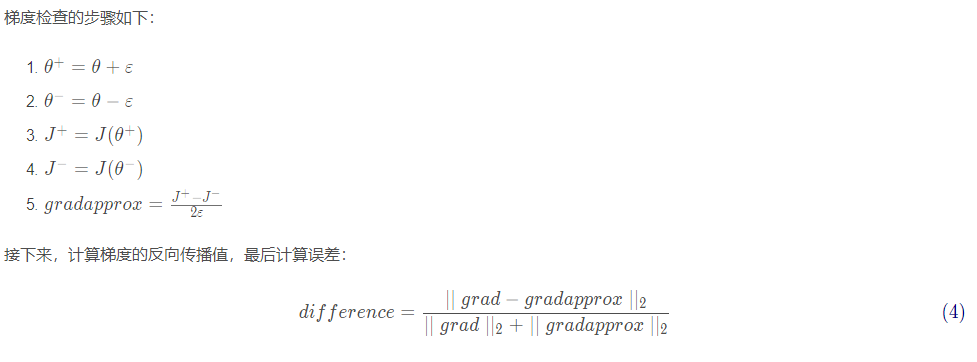
When the gradient detection formula is defined and the difference is less than the negative 7th power of 10, we usually think that our calculation result is correct.
def gradient_check(x,theta,epsilon=1e-7):
    """

    Implement the back propagation in the diagram.

    Parameters:
        x  - A real value input
        theta  - Parameter is also a real number
        epsilon  - Use equation (3) to calculate the small offset of the input to calculate the approximate gradient

    return:
        Difference between approximate gradient and backward propagation gradient
    """

    #Calculate gradaprox using the left side of equation (3).
    thetaplus = theta + epsilon                               # Step 1
    thetaminus = theta - epsilon                              # Step 2
    J_plus = forward_propagation(x, thetaplus)                # Step 3
    J_minus = forward_propagation(x, thetaminus)              # Step 4
    gradapprox = (J_plus - J_minus) / (2 * epsilon)           # Step 5


    #Check that gradaprox is close enough to backward_ Output of propagation()
    grad = backward_propagation(x, theta)

    numerator = np.linalg.norm(grad - gradapprox)                      # Step 1'
    denominator = np.linalg.norm(grad) + np.linalg.norm(gradapprox)    # Step 2'
    difference = numerator / denominator                               # Step 3'

    if difference < 1e-7:
        print("Gradient inspection: the gradient is normal!")
    else:
        print("Gradient check: gradient exceeds threshold!")

    return difference
Forward propagation in high dimensional case
def forward_propagation_n(X,Y,parameters):
    """
    Realize the forward propagation in the diagram (and calculate the cost).

    Parameters:
        X - Training set is m Examples
        Y -  m Label for example
        parameters - Include parameters“ W1","b1","W2","b2","W3","b3"of python Dictionaries:
            W1  - Weight matrix with dimension (5),4)
            b1  - Bias, dimension (5),1)
            W2  - Weight matrix with dimension (3),5)
            b2  - Bias, dimension (3),1)
            W3  - Weight matrix with dimension (1),3)
            b3  - Bias, dimension (1),1)

    return:
        cost - Cost function( logistic)
    """
    m = X.shape[1]
    W1 = parameters["W1"]
    b1 = parameters["b1"]
    W2 = parameters["W2"]
    b2 = parameters["b2"]
    W3 = parameters["W3"]
    b3 = parameters["b3"]

    # LINEAR -> RELU -> LINEAR -> RELU -> LINEAR -> SIGMOID
    Z1 = np.dot(W1,X) + b1
    A1 = gc_utils.relu(Z1)

    Z2 = np.dot(W2,A1) + b2
    A2 = gc_utils.relu(Z2)

    Z3 = np.dot(W3,A2) + b3
    A3 = gc_utils.sigmoid(Z3)

    #Calculate cost
    logprobs = np.multiply(-np.log(A3), Y) + np.multiply(-np.log(1 - A3), 1 - Y)
    cost = (1 / m) * np.sum(logprobs)

    cache = (Z1, A1, W1, b1, Z2, A2, W2, b2, Z3, A3, W3, b3)

    return cost, cache
Back propagation
def backward_propagation_n(X,Y,cache):
    """
    Implement the back propagation shown in the figure.

    Parameters:
        X - Input data points (number of input nodes, 1)
        Y - label
        cache - come from forward_propagation_n()of cache output

    return:
        gradients - A dictionary containing cost gradients associated with each parameter, activation, and pre activation variable.
    """
    m = X.shape[1]
    (Z1, A1, W1, b1, Z2, A2, W2, b2, Z3, A3, W3, b3) = cache

    dZ3 = A3 - Y
    dW3 = (1. / m) * np.dot(dZ3,A2.T)
    dW3 = 1. / m * np.dot(dZ3, A2.T)
    db3 = 1. / m * np.sum(dZ3, axis=1, keepdims=True)

    dA2 = np.dot(W3.T, dZ3)
    dZ2 = np.multiply(dA2, np.int64(A2 > 0))
    #dW2 = 1. / m * np.dot(dZ2, A1.T) * 2  # Should not multiply by 2
    dW2 = 1. / m * np.dot(dZ2, A1.T)
    db2 = 1. / m * np.sum(dZ2, axis=1, keepdims=True)

    dA1 = np.dot(W2.T, dZ2)
    dZ1 = np.multiply(dA1, np.int64(A1 > 0))
    dW1 = 1. / m * np.dot(dZ1, X.T)
    #db1 = 4. / m * np.sum(dZ1, axis=1, keepdims=True) # Should not multiply by 4
    db1 = 1. / m * np.sum(dZ1, axis=1, keepdims=True)

    gradients = {"dZ3": dZ3, "dW3": dW3, "db3": db3,
                 "dA2": dA2, "dZ2": dZ2, "dW2": dW2, "db2": db2,
                 "dA1": dA1, "dZ1": dZ1, "dW1": dW1, "db1": db1}

    return gradients
The gradient test formula in the high-dimensional case is the same as the one-dimensional linear formula, but, θ It's no longer a scalar. It's a dictionary called "parameters". In the required database, we implemented a function "dictionary_to_vector()" for you. It converts the "parameter" dictionary into a vector called "value", which is obtained by reshaping all parameters (W1, b1, W2, b2, W3, b3) into vectors and concatenating them. The inverse function is "vector_to_dictionary" , which outputs back to the "parameters" dictionary.
Define n-dimensional gradient test function
def gradient_check_n(parameters,gradients,X,Y,epsilon=1e-7):
    """
    inspect backward_propagation_n Is it calculated correctly forward_propagation_n Output cost gradient

    Parameters:
        parameters - Include parameters“ W1","b1","W2","b2","W3","b3"of python Dictionaries:
        grad_output_propagation_n The output of contains the cost gradient associated with the parameter.
        x  - Enter the data point with dimension (enter the number of nodes, 1)
        y  - label
        epsilon  - Calculate the small offset of the input to calculate the approximate gradient

    return:
        difference - Difference between approximate gradient and backward propagation gradient
    """
    #Initialization parameters
    parameters_values , keys = gc_utils.dictionary_to_vector(parameters) #keys not available
    grad = gc_utils.gradients_to_vector(gradients)
    num_parameters = parameters_values.shape[0]
    J_plus = np.zeros((num_parameters,1))
    J_minus = np.zeros((num_parameters,1))
    gradapprox = np.zeros((num_parameters,1))

    #Calculate gradaprox
    for i in range(num_parameters):
        #Calculate J_plus [i]. Input: "parameters_values, epsilon". Output = "J_plus [i]"
        thetaplus = np.copy(parameters_values)                                                  # Step 1
        thetaplus[i][0] = thetaplus[i][0] + epsilon                                             # Step 2
        J_plus[i], cache = forward_propagation_n(X,Y,gc_utils.vector_to_dictionary(thetaplus))  # Step 3, the cache is not used

        #Calculate J_minus [i]. Input: "parameters_values, epsilon". Output = "J_minus [i]".
        thetaminus = np.copy(parameters_values)                                                 # Step 1
        thetaminus[i][0] = thetaminus[i][0] - epsilon                                           # Step 2
        J_minus[i], cache = forward_propagation_n(X,Y,gc_utils.vector_to_dictionary(thetaminus))# Step 3, the cache is not used

        #Calculate gradaprox [i]
        gradapprox[i] = (J_plus[i] - J_minus[i]) / (2 * epsilon)

    #Gradaprox and backward propagation gradients are compared by calculating the difference.
    numerator = np.linalg.norm(grad - gradapprox)                                     # Step 1'
    denominator = np.linalg.norm(grad) + np.linalg.norm(gradapprox)                   # Step 2'
    difference = numerator / denominator                                              # Step 3'

    if difference < 1e-7:
        print("Gradient inspection: the gradient is normal!")
    else:
        print(difference,"Gradient check: gradient exceeds threshold!")

    return difference
Verify the gradient test results in multi-dimensional case
#Functions in testCases in the data file
X, Y, parameters = gradient_check_n_test_case()

cost, cache = forward_propagation_n(X, Y, parameters)
gradients = backward_propagation_n(X, Y, cache)
difference = gradient_check_n(parameters, gradients, X, Y)
Finally, the running results of multidimensional gradient test

Gradient test complete code
import numpy as np
import matplotlib.pyplot as plt
import reg_utils
import gc_utils
from reg_utils import sigmoid, relu, plot_decision_boundary, initialize_parameters, load_2D_dataset, predict_dec
from reg_utils import compute_cost, predict, forward_propagation, backward_propagation, update_parameters
import sklearn
import sklearn.datasets
import scipy.io
from testCases import *

# Forward propagation of one-dimensional linear model
def forward_propagation(x, theta):
    """

    Realize the linear forward propagation (calculation) presented in the figure J)(J(theta)= theta * x)

    Parameters:
    x  - A real value input
    theta  - Parameter is also a real number

    return:
    J  - function J Value of, using formula J(theta)= theta * x calculation
    """
    J = np.dot(theta, x)

    return J

#Back propagation
def backward_propagation(x, theta):
    """
    calculation J be relative toθDerivative of.

    Parameters:
        x  - A real value input
        theta  - Parameter is also a real number

    return:
        dtheta  - be relative toθCost gradient
    """
    dtheta = x

    return dtheta
# One dimensional linear gradient test function
def gradient_check(x, theta, epsilon=1e-7):
    """

    Implement the back propagation in the diagram.

    Parameters:
        x  - A real value input
        theta  - Parameter is also a real number
        epsilon  - Use equation (3) to calculate the small offset of the input to calculate the approximate gradient

    return:
        Difference between approximate gradient and backward propagation gradient
    """

    # Calculate gradaprox using the left side of equation (3).
    thetaplus = theta + epsilon  # Step 1
    thetaminus = theta - epsilon  # Step 2
    J_plus = forward_propagation(x, thetaplus)  # Step 3
    J_minus = forward_propagation(x, thetaminus)  # Step 4
    gradapprox = (J_plus - J_minus) / (2 * epsilon)  # Step 5

    # Check that gradaprox is close enough to the output of backward_propagation()
    grad = backward_propagation(x, theta)

    numerator = np.linalg.norm(grad - gradapprox)  # Step 1'
    denominator = np.linalg.norm(grad) + np.linalg.norm(gradapprox)  # Step 2'
    difference = numerator / denominator  # Step 3'

    if difference < 1e-7:
        print("Gradient inspection: the gradient is normal!")
    else:
        print("Gradient check: gradient exceeds threshold!")

    return difference

# Test run results
# print("------------------ test gradient_check ---------------")
# x, theta = 2, 4
# difference = gradient_check(x, theta)
# print("difference = " + str(difference))

# Define multidimensional forward propagation
def forward_propagation_n(X, Y, parameters):
    """
    Realize the forward propagation in the diagram (and calculate the cost).

    Parameters:
        X - Training set is m Examples
        Y -  m Label for example
        parameters - Include parameters“ W1","b1","W2","b2","W3","b3"of python Dictionaries:
            W1  - Weight matrix with dimension (5),4)
            b1  - Bias, dimension (5),1)
            W2  - Weight matrix with dimension (3),5)
            b2  - Bias, dimension (3),1)
            W3  - Weight matrix with dimension (1),3)
            b3  - Bias, dimension (1),1)

    return:
        cost - Cost function( logistic)
    """
    m = X.shape[1]
    W1 = parameters["W1"]
    b1 = parameters["b1"]
    W2 = parameters["W2"]
    b2 = parameters["b2"]
    W3 = parameters["W3"]
    b3 = parameters["b3"]

    # LINEAR -> RELU -> LINEAR -> RELU -> LINEAR -> SIGMOID
    Z1 = np.dot(W1, X) + b1
    A1 = gc_utils.relu(Z1)

    Z2 = np.dot(W2, A1) + b2
    A2 = gc_utils.relu(Z2)

    Z3 = np.dot(W3, A2) + b3
    A3 = gc_utils.sigmoid(Z3)

    # Calculate cost
    logprobs = np.multiply(-np.log(A3), Y) + np.multiply(-np.log(1 - A3), 1 - Y)
    cost = (1 / m) * np.sum(logprobs)

    cache = (Z1, A1, W1, b1, Z2, A2, W2, b2, Z3, A3, W3, b3)

    return cost, cache

# Multidimensional back propagation
def backward_propagation_n(X, Y, cache):
    """
    Implement the back propagation shown in the figure.

    Parameters:
        X - Input data points (number of input nodes, 1)
        Y - label
        cache - come from forward_propagation_n()of cache output

    return:
        gradients - A dictionary containing cost gradients associated with each parameter, activation, and pre activation variable.
    """
    m = X.shape[1]
    (Z1, A1, W1, b1, Z2, A2, W2, b2, Z3, A3, W3, b3) = cache

    dZ3 = A3 - Y
    dW3 = (1. / m) * np.dot(dZ3, A2.T)
    dW3 = 1. / m * np.dot(dZ3, A2.T)
    db3 = 1. / m * np.sum(dZ3, axis=1, keepdims=True)

    dA2 = np.dot(W3.T, dZ3)
    dZ2 = np.multiply(dA2, np.int64(A2 > 0))
    # dW2 = 1. / m * np.dot(dZ2, A1.T) * 2  # Should not multiply by 2
    dW2 = 1. / m * np.dot(dZ2, A1.T)
    db2 = 1. / m * np.sum(dZ2, axis=1, keepdims=True)

    dA1 = np.dot(W2.T, dZ2)
    dZ1 = np.multiply(dA1, np.int64(A1 > 0))
    dW1 = 1. / m * np.dot(dZ1, X.T)
    # db1 = 4. / m * np.sum(dZ1, axis=1, keepdims=True) # Should not multiply by 4
    db1 = 1. / m * np.sum(dZ1, axis=1, keepdims=True)

    gradients = {"dZ3": dZ3, "dW3": dW3, "db3": db3,
                 "dA2": dA2, "dZ2": dZ2, "dW2": dW2, "db2": db2,
                 "dA1": dA1, "dZ1": dZ1, "dW1": dW1, "db1": db1}

    return gradients

# Multidimensional gradient test function
def gradient_check_n(parameters, gradients, X, Y, epsilon=1e-7):
    """
    inspect backward_propagation_n Is it calculated correctly forward_propagation_n Output cost gradient

    Parameters:
        parameters - Include parameters“ W1","b1","W2","b2","W3","b3"of python Dictionaries:
        grad_output_propagation_n The output of contains the cost gradient associated with the parameter.
        x  - Enter the data point with dimension (enter the number of nodes, 1)
        y  - label
        epsilon  - Calculate the small offset of the input to calculate the approximate gradient

    return:
        difference - Difference between approximate gradient and backward propagation gradient
    """
    # Initialization parameters
    parameters_values, keys = gc_utils.dictionary_to_vector(parameters)  # keys not available
    grad = gc_utils.gradients_to_vector(gradients)
    num_parameters = parameters_values.shape[0]
    J_plus = np.zeros((num_parameters, 1))
    J_minus = np.zeros((num_parameters, 1))
    gradapprox = np.zeros((num_parameters, 1))

    # Calculate gradaprox
    for i in range(num_parameters):
        # Calculate J_plus [i]. Input: "parameters_values, epsilon". Output = "J_plus [i]"
        thetaplus = np.copy(parameters_values)  # Step 1
        thetaplus[i][0] = thetaplus[i][0] + epsilon  # Step 2
        J_plus[i], cache = forward_propagation_n(X, Y, gc_utils.vector_to_dictionary(thetaplus))  # Step 3, the cache is not used

        # Calculate J_minus [i]. Input: "parameters_values, epsilon". Output = "J_minus [i]".
        thetaminus = np.copy(parameters_values)  # Step 1
        thetaminus[i][0] = thetaminus[i][0] - epsilon  # Step 2
        J_minus[i], cache = forward_propagation_n(X, Y, gc_utils.vector_to_dictionary(thetaminus))  # Step 3, the cache is not used

        # Calculate gradaprox [i]
        gradapprox[i] = (J_plus[i] - J_minus[i]) / (2 * epsilon)

    # Gradaprox and backward propagation gradients are compared by calculating the difference.
    numerator = np.linalg.norm(grad - gradapprox)  # Step 1'
    denominator = np.linalg.norm(grad) + np.linalg.norm(gradapprox)  # Step 2'
    difference = numerator / denominator  # Step 3'

    if difference < 1e-7:
        print("Gradient inspection: the gradient is normal!")
    else:
        print(difference,"Gradient check: gradient exceeds threshold!")

    return difference

# Operation gradient test results

#Functions in testCases in the data file
X, Y, parameters = gradient_check_n_test_case()

cost, cache = forward_propagation_n(X, Y, parameters)
gradients = backward_propagation_n(X, Y, cache)
difference = gradient_check_n(parameters, gradients, X, Y)
Summary
Gradient test is slow! Approaching the gradient is computationally expensive. Therefore, we will not perform gradient test in each iteration during training. Just check whether the gradient is correct several times. Gradient test is not applicable to dropout. Generally, you will run the gradient test algorithm without dropout to ensure that your back propagation is correct, and then add dropout.