Network Overview (Thesis)

Related paper resources: in my resources, please pay attention to me and then download. There are three papers:

1. Deep Subspace Clustering Networks
2. Deep Multimodal Subspace Clustering Networks
3. Cross-Modal Subspace Clustering via Deep Canonical Correlation Analysis

Next, we will explain the multimodal subspace clustering network.

introduction

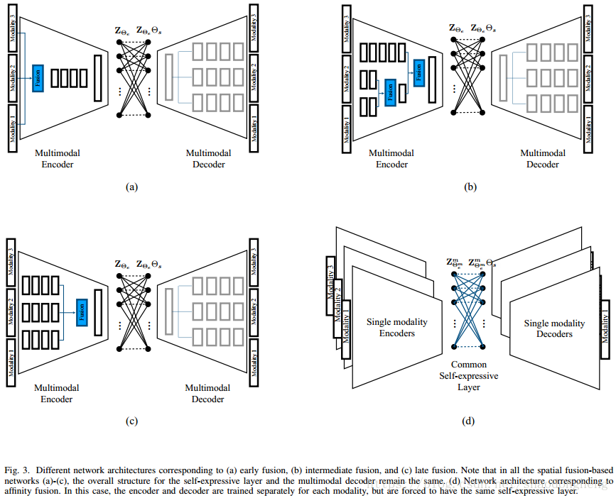
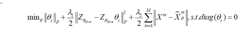
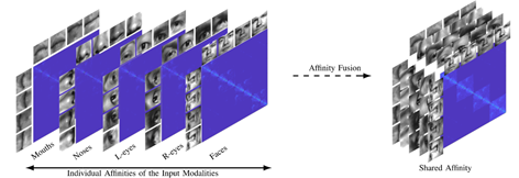
Deep multimodal subspace clustering network (DMSC) is mainly composed of encoder, decoder and self-expression layer. Each mode corresponds to its own encoder and decoder, and the parameters are not shared. The network structure is shown in the figure:

The training process of the model is divided into two steps: in the first step, the self coding network structure composed of encoder and decoder is used to train the function of multi-modal data mapping to subspace and spatial fusion. The output of the network is that the decoder is reconstructed from the potential space to keep consistent with the source multi-modal data as much as possible; The loss function of the network is the distance between the reconstruction of the decoder and the original input, and the loss function is continuously minimized through training. The second step is to add a self-expression layer on the basis of the first step. The self-expression layer is based on bipartite graph neural network, and the parameters of the self-expression layer represent the affinity matrix of the similarity between the training samples. Encoder network for early fusion, late fusion and hybrid fusion, three encoder networks for different spatial fusion methods are proposed. Different fusion methods have no effect on the self-expression layer and multimodal decoder. In addition to these three spatial fusion methods, a network based on affinity fusion is also proposed. In the affinity fusion method, the self-expression layer is shared among modes in this fusion network.
The network model has the following advantages:

1. A multi-mode subspace clustering framework based on deep learning is proposed
   Encoding self representation attributes in subspace.
2. Aiming at the fusion of multimodal data, a new encoder corresponding to late, early and intermediate fusion is proposed
   Network architecture.
3. A network architecture based on affinity fusion is proposed. In this architecture, the self-expression layer is strong
   The system has the same weight for the subspace features of all modes.

Deep Subspace Clustering Networks (deep subspace clustering based on sparse and low rank representation)

Vector order X = [ x 1 , ... , x N ] ∈ R ( D × N ) X=[x_1,...,x_N]∈R^{(D×N)} X=[x1​,…,xN​]∈R(D × N) Is from R D R^D Dimension in RD is d l ( l = 1 ) n {d_l}_{(l=1)}^n N linear subspaces s of dl (l=1)n +_ 1∪S_2∪…S_ The union of N draws the set of N signals. Given X, find at S l S_l Submatrix of Sl + X l ∈ R ( D × N l ) X_l∈R^{(D×N_l )} Xl​∈R(D × Nl) is the main task of subspace clustering, in which N 1 + N 2 + ⋯ + N n = N . N_1+N_2+⋯+N_n=N. N1​+N2​+⋯+Nn​=N. Assuming that each data sample can be represented by a linear combination of other data points, the purpose of these algorithms is to find a sparse or low rank matrix C by solving the optimization problem of formula (4-1):
m i n ∣ ∣ C ∣ ∣ p + λ / 2 ∣ ∣ X − X C ∣ ∣ F 2 min||C||_p+\lambda/2||X-XC||_F^2 min∣∣C∣∣p​+λ/2∣∣X−XC∣∣F2​
Of which ||| Means solving the norm, λ Represents the regularization parameter. In addition, in order to prevent the general solution C=I, I is the identity matrix, the diagonal value is 1, and the others are all 0. Will the above d i a g ( C ) = 0 diag(C)=0 The additional constraint of diag(C)=0 is added to the above optimization problem. Once C is found, the spectral clustering method is applied to the obtained affinity matrix W, W = ∣ C ∣ + ∣ C ∣ T W=|C|+|C|^T W = ∣ C ∣ + ∣ C ∣ T, so as to obtain the segmentation and clustering results of dataset X.
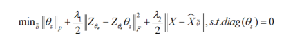
The data set X represented in the subspace is a deep subspace clustering network, which explores self-expression by embedding data into potential space using encoder decoder type network. Figure 4.2 is an overview of deep subspace clustering of single-mode subspace clustering. This method uses the trainable dense layer embedded in the network to approximate matrix C, and the parameters of the self-expression layer are expressed as θ s θ_s θ s, using the loss function formula, the following function is used to train the network:

among Z ( θ e ) Z_{(θ_e )} Z( θ e) represents the output of the encoder, X θ X_{θ} X θ Is the reconstructed signal at the output of the decoder. Here, network parameters θ By encoder parameters θ_ e and self-expression layer parameters θ_ s composition. here, λ 1 λ_1 λ 1. And λ 2 λ_2 λ 2 ， are two regularization parameters.

Spectral clustering applied to the affinity matrix obtained by the network is an algorithm evolved from graph theory, which can also be called graph based clustering method, which is widely used in clustering. This method first calculates the similarity matrix, degree matrix and Laplace matrix between samples according to the given data set, then calculates the eigenvectors and Laplace eigenvalues, and finally selects the appropriate number of eigenvectors a and uses the traditional clustering algorithm. The elements in the degree matrix w i j w_ij wi j represents the distance and similarity between samples i and j. the purpose of clustering is to make the similarity of samples in the same cluster high and that of different clusters low.
Select the sample set before the algorithm starts D = x 1 , x 2 , ... , x n D={x_1,x_2,...,x_n} D=x1, x2,..., xn, algorithm for generating similarity matrix, clustering method, dimension after clustering k 2 k_2 k2 # and dimensionality after dimensionality reduction k 1 k_1 k1, the model will eventually output the divided data set of the cluster: C ( c 1 , c 2 , ... , c ( k 2 ) ) C(c_1,c_2,...,c_{(k_2 )}) C(c1​,c2​,...,c(k2​)​).
The basic flow of spectral clustering algorithm is as follows:

1. Calculate the adjacency matrix A and degree matrix (diagonal matrix) D of the sample set with the number of n;
2. Calculate Laplace matrix L=D-A;
3. Calculate the normalized Laplace matrix L = I − D ( 1 / 2 ) ∙ A ∙ D ( 1 / 2 ) L=I-D^{(1/2)}∙A∙D^{(1/2)} L=I−D(1/2)∙A∙D(1/2)；
4. Calculate the eigenvector Q of L and the corresponding eigenvalue, and select the smallest one k 1 k_1 Corresponding to k1# eigenvalues
   Eigenvector f of
5. The matrix composed of the corresponding eigenvectors f is normalized by rows to form n × k 1 n×k_1 n × k1 - dimensional characteristic matrix F;
6. Each line in F should have a dimension of k_1 samples, a total of n samples, using the input method for aggregation
   Class, the clustering dimension is k_2；
7. Get the clustering results C ( c 1 , c 2 , ... , c ( k 2 ) ) C(c_1,c_2,...,c_{(k_2 )}) C(c1​,c2​,...,c(k2​)​).

Compared with the traditional clustering algorithm, the deep clustering network has stronger generalization. It can be used not only for convex data, but also for arbitrary shape data space. But there are also some disadvantages: first, the dimensionality reduction operation has an obvious impact on the effect of clustering. Because the range of dimension reduction is not enough, it may lead to very high dimension in the final clustering. High dimension may lead to slow operation of spectral clustering algorithm and poor clustering effect. Secondly, different affinity matrices may lead to different final clustering effects.

Multi mode subspace clustering based on spatial fusion

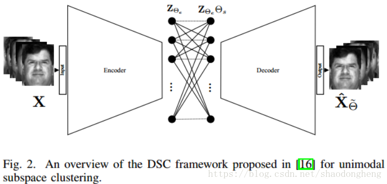
In video clustering, the unsupervised subspace clustering network based on spatial fusion is adopted by taking advantage of the characteristics that video is multimodal data. The purpose of spatial fusion method is to find a joint representation containing supplementary information from different modes. The joint representation has a corresponding relationship with each mode. The following figure shows multimodal spatial fusion:

An important part of this method is the fusion function f, which fuses the information from multiple input representations and returns the fusion output. In the case of deep network, the flexibility of fusion network selection leads to different models. Firstly, spatial fusion can be realized by using encoder in deep multimodal subspace clustering network, and then the fused expression becomes the input of self-expression layer, which uses the self-expression property of joint representation. Then, the multimodal decoder reconstructs different modes in the joint representation generated by the output of the self-expression layer.
For the case of M input modes, the decoder consists of M branches, and each branch reconstructs a mode. For multimodal fusion, the encoder can be designed to enable them to achieve early, late and hybrid fusion. As shown in the figure below, an overview of deep multimodal subspace clustering networks with different spatial fusion structures is given respectively. Early fusion refers to the stage of integrating multimodal data at the feature level before feeding it to the network. Late stage fusion involves the integration of multimodal data in the final stage of the network. The flexibility of deep network also provides a third kind of fusion called hybrid fusion, which can better fuse the intermediate coding features of encoder network. In all three cases, the structure of the multimodal decoder remains unchanged.

Assume that for specific data points x i x_i xi, there are M characteristic diagrams corresponding to the representations of different modes. Fusion function f : x 1 , x 2 , ... , x M → Z f:{x^1,x^2,...,x^M}→Z f:x1,x2,..., xM → Z fuse m feature maps and generate output Z. In order to make the representation more clear, this method assumes that all input feature maps have the same size R(H) × W × din), and the output has R(H) × W × dout). In fact, the deep network structure provides design options for feature maps with the same size. This is also the embodiment of the flexibility of depth network as a fusion function. The network uses z_(i,j,k) and x_(i,j,k)^m represents the spatial position (I, J, K) of the characteristic diagram of the m-th mode of output and input. The following describes various fusion functions commonly used to combine input feature mapping.

1. sum
2. maxpooling
3. concat

Given N paired data samples from M different modes ( X i 1 , X i 2 , ... , X i M ) ( i = 1 ) N (X_i^1,X_i^2,...,X_i^M)_{(i=1)}^N (Xi1, Xi2,..., XiM) (i=1)N, the corresponding m modal input data matrix is defined as X m = [ X 1 m , X s m , ... , X N m ] , m ∈ 1 , ... , M . X^m=[X_1^m,X_s^m,...,X_N^m],m∈{1,...,M}. Xm=[X1m​,Xsm​,…,XNm​],m∈1,…,M. Regardless of the network structure and the selected fusion function, let θ ( M ∙ e ) θ_{(M∙e)} θ (M ∙ e) represents the parameters of the multimode encoder. Similarly, make θ s θ_s θ s ， is a self-expression layer parameter, and θ ( M ⋅ d ) θ_{(M⋅d)} θ (M ⋅ d) is the parameter of multimodal decoder. Then, the following loss function is used to train the proposed spatial fusion function model end-to-end.

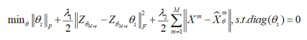
Deep multimodal subspace clustering based on affinity fusion

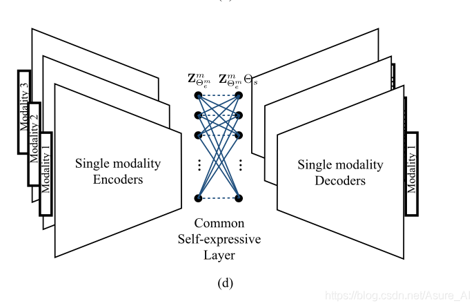
In addition to the multimodal fusion method of spatial fusion proposed in the previous section, the affinity fusion method can also be used to fuse the affinity between data models, so as to make the clustering effect better. The core idea of shared affinity matrix is that similar (dissimilar) data in one mode should also be similar (dissimilar) in other modes. Affinity fusion uses the similarity of self-expression to obtain the joint representation between multimodal data. The difference from spatial fusion is that the problem of data alignment does not need to be considered, because a mode is encoded by a completely independent encoder. The encoder is only responsible for subspace mapping of data, and there is no task of multi-modal fusion. Multimodal fusion is realized based on self-expression layer. The following figure shows an example of an affinity fusion method.
In the framework of deep subspace clustering, the affinity matrix can be calculated from the weight of self-expression layer: W = ∣ θ s T ∣ + ∣ θ s ∣ W=|θ_s^T |+|θ_s | W=∣ θ sT​∣+∣ θ s​∣. among θ s θ_s θ s corresponds to the self-expression layer weight learned by the end-to-end training strategy. Therefore, shared θ s θ_s θ s ， produce a common W in the whole mode. We enforce sharing θ s θ_s θ s ， modes with different encoders, decoders and potential representations at the same time.

For the network structure of multimodal clustering based on affinity fusion method, we stack M parallel deep subspace clustering networks, which share a common self-expression layer. In this model, an encoder decoder network is trained according to each mode. In contrast to the spatial fusion model, there is only one joint potential representation, which leads to M different potential representations corresponding to M different modes. Connect potential representations by sharing self-expression layers. The best self-expression layer should be able to make common use of self-expression attributes in all M modes. The following figure gives an overview of the proposed network architecture based on affinity fusion.

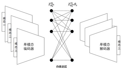
Find the shared self-expression weight by training the above network, and the loss function is shown in the formula:

Code explanation

Follow me to download the complete code in "my resources".

Model definition

The network includes a separate self coding network for each mode.

import torch.nn as nn
import torch
class Networks(nn.Module):
    def __init__(self):
        super(Networks, self).__init__()
        self.encoder1 = nn.Sequential(
            nn.Conv2d(1, 10, kernel_size=4, stride=2, padding=1, bias=True),#Grayscale image, channel 1
            nn.ReLU(),
            nn.Conv2d(10, 20, kernel_size=3, stride=1, padding=1, bias=True),
            nn.ReLU(),
            nn.Conv2d(20, 30, kernel_size=4, stride=2, padding=1, bias=True),
            nn.ReLU(),
        )
        self.decoder1 = nn.Sequential(
            nn.ConvTranspose2d(30, 20, kernel_size=4, stride=2, padding=1, bias=True),
            nn.ReLU(),
            nn.ConvTranspose2d(20, 10, kernel_size=3, stride=1, padding=1, bias=True),
            nn.ReLU(),
            nn.ConvTranspose2d(10, 1, kernel_size=4, stride=2, padding=0, bias=True),
            nn.ReLU(),
        )

        self.encoder2 = nn.Sequential(
            nn.Conv2d(1, 10, kernel_size=4, stride=2, padding=1, bias=True),
            nn.ReLU(),
            nn.Conv2d(10, 20, kernel_size=3, stride=1, padding=1, bias=True),
            nn.ReLU(),
            nn.Conv2d(20, 30, kernel_size=4, stride=2, padding=1, bias=True),
            nn.ReLU(),
        )
        self.decoder2 = nn.Sequential(
            nn.ConvTranspose2d(30, 20, kernel_size=4, stride=2, padding=1, bias=True),
            nn.ReLU(),
            nn.ConvTranspose2d(20, 10, kernel_size=3, stride=1, padding=1, bias=True),
            nn.ReLU(),
            nn.ConvTranspose2d(10, 1, kernel_size=4, stride=2, padding=0, bias=True),
            nn.ReLU(),
        )

        self.weight = nn.Parameter(1.0e-4 * torch.ones(2500, 2500))

    def forward(self, input1, input2):
        output1 = self.encoder1(input1)
        output1 = self.decoder1(output1)

        output2 = self.encoder2(input2)
        output2 = self.decoder2(output2)

        return output1, output2

    def forward2(self, input1, input2):#Self expression layer, get clustering
        coef = self.weight - torch.diag(torch.diag(self.weight))#Self expression layer parameters

        #Mode I
        z1 = self.encoder1(input1)
        z1 = z1.view(2500, 3000)#2500 individuals, 3000 dimensional characteristics
        zcoef1 = torch.matmul(coef, z1)#
        output1 = zcoef1.view(2500, 30, 10, 10)
        output1 = self.decoder1(output1)#decode
       #Mode II
        z2 = self.encoder2(input2)
        z2 = z2.view(2500, 3000)
        zcoef2 = torch.matmul(coef, z2)
        output2 = zcoef2.view(2500, 30, 10, 10)
        output2 = self.decoder2(output2)#decode

        return z1, z2, output1, output2, zcoef1, zcoef2, coef#Multimodal coded output, decoded output, layer 2 of self-expression layer, affinity matrix

model training

import torch
from data.dataloader import data_loader_train
from models.network import Networks
import models.metrics as metrics
import numpy as np
import scipy.io as sio
from scipy.sparse.linalg import svds
from sklearn import cluster
from sklearn.preprocessing import normalize


def thrC(C,ro):
    if ro < 1:
        N = C.shape[1]
        Cp = np.zeros((N,N))
        S = np.abs(np.sort(-np.abs(C),axis=0))
        Ind = np.argsort(-np.abs(C),axis=0)
        for i in range(N):
            cL1 = np.sum(S[:,i]).astype(float)
            stop = False
            csum = 0
            t = 0
            while(stop == False):
                csum = csum + S[t,i]
                if csum > ro*cL1:
                    stop = True
                    Cp[Ind[0:t+1,i],i] = C[Ind[0:t+1,i],i]
                t = t + 1
    else:
        Cp = C

    return Cp


def post_proC(C, K, d=6, alpha=8):#Spectral clustering
    # C: coefficient matrix, K: number of clusters, d: dimension of each subspace
    C = 0.5*(C + C.T)
    r = d*K + 1
    U, S, _ = svds(C,r,v0 = np.ones(C.shape[0]))
    U = U[:,::-1]
    S = np.sqrt(S[::-1])
    S = np.diag(S)
    U = U.dot(S)
    U = normalize(U, norm='l2', axis = 1)
    Z = U.dot(U.T)
    Z = Z * (Z>0)
    L = np.abs(Z ** alpha)
    L = L/L.max()
    L = 0.5 * (L + L.T)
    spectral = cluster.SpectralClustering(n_clusters=K, eigen_solver='arpack', affinity='precomputed',assign_labels='discretize')
    spectral.fit(L)
    grp = spectral.fit_predict(L) + 1
    return grp, L


data_0 = sio.loadmat('BDGP/label.mat')
data_dict = dict(data_0)
data0 = data_dict['groundtruth'].T
label_true = np.zeros(2500)
for i in range(2500):
    label_true[i] = data0[i]
print(label_true)# Load data label

reg2 = 1.0 * 10 ** (5 / 10.0 - 3.0)

model = Networks().cuda()
model.load_state_dict(torch.load('./models/AE1.pth'))#Model loading training model

criterion = torch.nn.MSELoss(reduction='sum')#loss function 
optimizer = torch.optim.Adam(filter(lambda p: p.requires_grad, model.parameters()), lr=0.001, weight_decay=0.0)#optimizer
n_epochs = 2000
for epoch in range(n_epochs):
    for data in data_loader_train:
        train_imga, train_imgb = data
        input1 = train_imga.view(2500, 1, 42, 42).cuda()
        input2 = train_imgb.view(2500, 1, 42, 42).cuda()
        output1, output2 = model(input1, input2)#Self coding network model training
        loss = 0.2 * criterion(output1, input1) + 0.8 * criterion(output2, input2)
        optimizer.zero_grad()
        loss.backward()
        optimizer.step()
    if epoch % 100 == 0:
        print("Epoch {}/{}".format(epoch, n_epochs))
        print("Loss is:{:.4f}".format(loss.item()))
torch.save(model.state_dict(), './models/AE1.pth')

print("step2")#Stage 2 training self expression layer
print("---------------------------------------")
criterion2 = torch.nn.MSELoss(reduction='sum')
optimizer2 = torch.optim.Adam(filter(lambda p: p.requires_grad, model.parameters()), lr=0.001, weight_decay=0.0)
n_epochs2 = 1001
for epoch in range(n_epochs2):
    for data in data_loader_train:
        train_imga, train_imgb = data
        input1 = train_imga.view(2500, 1, 42, 42).cuda()
        input2 = train_imgb.view(2500, 1, 42, 42).cuda()
        z1, z2, output1, output2, zcoef1, zcoef2, coef = model.forward2(input1, input2)#Output of self-expression layer
        #Multimodal coded output, decoded output, layer 2 of self-expression layer, affinity matrix
        loss_re = criterion2(coef, torch.zeros(2500, 2500, requires_grad=True).cuda())#A norm of self expression
        loss_e = 0.8 * criterion2(zcoef2, z2) + 0.2 * criterion2(zcoef1, z1)#Loss of self-expression of two modes
        loss_r = 0.2 * criterion2(output1, input1) + 0.8 * criterion2(output2, input2)#Self coding loss
        loss = loss_r + 0.1 * loss_re + 50 * reg2 * loss_e
        optimizer2.zero_grad()
        loss.backward()
        optimizer2.step()
    if epoch % 100 == 0:
        print("Epoch {}/{}".format(epoch, n_epochs2))
        print("Loss is:{:.4f}".format(loss.item()))
        coef = model.weight - torch.diag(torch.diag(model.weight))
        commonZ = coef.cpu().detach().numpy()
        alpha = max(0.4 - (5 - 1) / 10 * 0.1, 0.1)
        commonZ = thrC(commonZ, alpha)
        preds, _ = post_proC(commonZ, 5)
        acc = metrics.acc(label_true, preds)
        nmi = metrics.nmi(label_true, preds)
        print(' ' * 8 + '|==>  acc: %.4f,  nmi: %.4f  <==|'
              % (acc, nmi))
        Z_path = 'commonZ' + str(epoch)
        sio.savemat(Z_path + '.mat', {'Z': commonZ})
torch.save(model.state_dict(), './models/AE2.pth')#Save the trained model file