DenseNet, a densely connected convolution network with Pytorch Note32
A summary of all notes: Pytorch Note Happy Planet
DenseNet
Previous Resnet enhanced the information flow between the front and back layers through Shortcuts, alleviated the disappearance of gradients to some extent, and built the neural network very deeply. Furthermore, DenseNet maximizes this kind of front-back information exchange by creating dense connections between all the front-front layers and the back-end layers, enabling the reuse of features on the channel dimension to achieve better performance than ResNet with fewer parameters and computations. If you want to learn more about and view your paper, you can read another of my blogs DenseNet: Densely Connected Convolutional Network
DenseNet differs from ResNet in that ResNet is a cross-layer summation, whereas DenseNet splits features across the channel dimensions, as illustrated below.
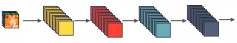
This is the most standard convolution neural network
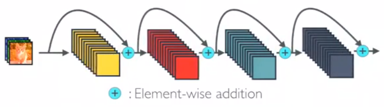
This is ResNet, a cross-layer summation

This is DenseNet, which splices features across channels
Dense Block
The network architecture of DenseNet is illustrated below. To facilitate the implementation of downsampling, we divide the network into dense blocks with dense connections. The network is composed of several Dense Blocks and a convolution pool in the middle, the core of which is in Dense Block. The black dots in Dense Block represent a convolution layer, where multiple black lines represent the flow of data, and each layer's input consists of the output of all previous convolutions. Note that the Concatnate operation is used instead of ResNet's element-by-element addition operation.
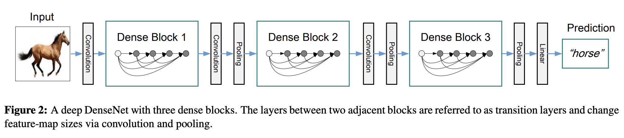
We call the layer between each block a transition layer to complete convolution and pooling. In our experiment, the transition layer is composed of BN layer, 1x1 convolution layer and 2x2 average pooling layer.
Details of the Block implementation are shown below, and each Block consists of several convolution layers of Bottleneck corresponding to the black dots in the figure above. Bottleneck by BN, ReLU, 1 × 1 Convolution, BN, ReLU, 3 × 3 The order of the convolution, also known as the DenseNet-B structure. Among them, 1x1 Conv produces 4k feature maps. It reduces the number of features and improves computational efficiency.

There are four details to note about Block:
- The number of signature channels for each Bottleneck output is the same, for example, 32 here. You can also see that the number of channels after Concatnate operation increases by 32, so this 32 is also known as GrowthRate.
- Here 1 × 1 Convolution works by fixing the number of output channels to reduce dimensionality. When dozens of Bottleneck s are connected, the number of channels behind Concatnate increases to thousands, if not 1 × Convolution of 1 to reduce dimensions, followed by 3 × 3 The amount of parameters required for convolution increases dramatically. 1 × 1 The number of convoluted channels is usually four times that of GrowthRate.
- In the above diagram, the feature is passed directly from the feature Concatnate of all the previous layers to the next layer, which is consistent with how the specific code is implemented.
- Block uses the order of activation function before and convolution layer after, which is different from the general network.
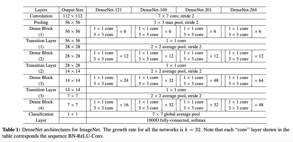
Network Structure of DenseNet
The network on the ImageNet dataset is shown below
code implementation
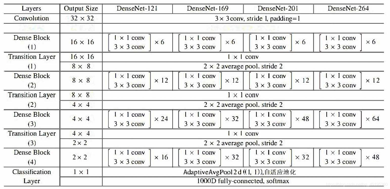
Because I'm experimenting with CIFAR and ImageNet's network model is given in this paper, the model is slightly different due to different datasets
Bottleneck
class Bottleneck(nn.Module):
    """
    Dense Block
    There growth_rate=out_channels, Is Every Block Number of channels output by oneself.
    Pass 1 first x1 Convolution layer, reducing the number of channels to 4 * growth_rate,Then go through 3 x3 Convolution layer down to growth_rate.
    """
    # Usually 1 × 1 The convoluted number of channels is four times that of GrowthRate
    expansion = 4

    def __init__(self, in_channels, growth_rate):
        super(Bottleneck, self).__init__()
        zip_channels = self.expansion * growth_rate
        self.features = nn.Sequential(
            nn.BatchNorm2d(in_channels),
            nn.ReLU(True),
            nn.Conv2d(in_channels, zip_channels, kernel_size=1, bias=False),
            nn.BatchNorm2d(zip_channels),
            nn.ReLU(True),
            nn.Conv2d(zip_channels, growth_rate, kernel_size=3, padding=1, bias=False)
        )

    def forward(self, x):
        out = self.features(x)
        out = torch.cat([out, x], 1)
        return out
Transition
class Transition(nn.Module):
    """
    Dimensionally changing Transition Layer Specifically Includes BN,ReLU,1×1 Convolution ( Conv),2×2 Average pooling operation
    Pass 1 first x1 Decrease in convolution channels,Pass 2 x2 Average pooling layer reduction feature-map
    """
    # 1 × 1 Convolution reduces dimensionality and compresses the model, while average pooling reduces the size of the signature graph.
    def __init__(self, in_channels, out_channels):
        super(Transition, self).__init__()
        self.features = nn.Sequential(
            nn.BatchNorm2d(in_channels),
            nn.ReLU(True),
            nn.Conv2d(in_channels, out_channels, kernel_size=1, bias=False),
            nn.AvgPool2d(2)
        )

    def forward(self, x):
        out = self.features(x)
        return out
DenseNet
# DesneNet-BC
# B stands for bottleneck layer(BN-RELU-CONV(1x1)-BN-RELU-CONV(3x3))
# C stands for compression factor (0<=theta<=1)
import math
class DenseNet(nn.Module):
    """
    Dense Net
    paper in growth_rate Take 12, the parameter for dimension compressionθ,That is reduction Take 0.5
    And the initialization method is kaiming_normal()
    num_blocks For each segment of the network DenseBlock Number
    DenseNet and ResNet It's also a six-segment network (a convolution)+Four Segments Dense+Average pooling layer), last FC Layer.
    The first paragraph changes the dimension from 3 to 2 * growth_rate

    (3, 32, 32) -> [Conv2d] -> (24, 32, 32) -> [layer1] -> (48, 16, 16) -> [layer2]
  ->(96, 8, 8) -> [layer3] -> (192, 4, 4) -> [layer4] -> (384, 4, 4) -> [AvgPool]
  ->(384, 1, 1) -> [Linear] -> (10)

    """
    def __init__(self, num_blocks, growth_rate=12, reduction=0.5, num_classes=10):
        super(DenseNet, self).__init__()
        self.growth_rate = growth_rate
        self.reduction = reduction

        num_channels = 2 * growth_rate

        self.features = nn.Conv2d(3, num_channels, kernel_size=3, padding=1, bias=False)
        self.layer1, num_channels = self._make_dense_layer(num_channels, num_blocks[0])
        self.layer2, num_channels = self._make_dense_layer(num_channels, num_blocks[1])
        self.layer3, num_channels = self._make_dense_layer(num_channels, num_blocks[2])
        self.layer4, num_channels = self._make_dense_layer(num_channels, num_blocks[3], transition=False)
        self.avg_pool = nn.Sequential(
            nn.BatchNorm2d(num_channels),
            nn.ReLU(True),
            nn.AvgPool2d(4),
        )
        self.classifier = nn.Linear(num_channels, num_classes)

        self._initialize_weight()

    def _make_dense_layer(self, in_channels, nblock, transition=True):
        layers = []
        for i in range(nblock):
            layers += [Bottleneck(in_channels, self.growth_rate)]
            in_channels += self.growth_rate
        out_channels = in_channels
        if transition:
            out_channels = int(math.floor(in_channels * self.reduction))
            layers += [Transition(in_channels, out_channels)]
        return nn.Sequential(*layers), out_channels

    def _initialize_weight(self):
        for m in self.modules():
            if isinstance(m, nn.Conv2d):
                nn.init.kaiming_normal_(m.weight.data)
                if m.bias is not None:
                    m.bias.data.zero_()

    def forward(self, x):
        out = self.features(x)
        out = self.layer1(out)
        out = self.layer2(out)
        out = self.layer3(out)
        out = self.layer4(out)
        out = self.avg_pool(out)
        out = out.view(out.size(0), -1)
        out = self.classifier(out)
        return out
def DenseNet121():
    return DenseNet([6,12,24,16], growth_rate=32)

def DenseNet169():
    return DenseNet([6,12,32,32], growth_rate=32)

def DenseNet201():
    return DenseNet([6,12,48,32], growth_rate=32)

def DenseNet161():
    return DenseNet([6,12,36,24], growth_rate=48)

def densenet_cifar():
    return DenseNet([6,12,24,16], growth_rate=12)

net = DenseNet121().to(device)
Now you can test it
# test
x = torch.randn(2, 3, 32, 32).to(device)
y = net(x)
print(y.shape)
torch.Size([2, 10])
As you can see, there is no problem, and then I'll classify DenseNet121 into images for our CIFAR-10 data
from utils import train
from utils import plot_history
Acc, Loss, Lr = train(net, trainloader, testloader, epoch, optimizer, criterion, scheduler, save_path, verbose = True)
Epoch [  1/ 20]  Train Loss:1.457685  Train Acc:46.79% Test Loss:1.159939  Test Acc:58.61%  Learning Rate:0.100000	Time 03:26
Epoch [  2/ 20]  Train Loss:0.918042  Train Acc:67.23% Test Loss:0.978080  Test Acc:66.76%  Learning Rate:0.100000	Time 03:26
Epoch [  3/ 20]  Train Loss:0.713618  Train Acc:75.13% Test Loss:0.702649  Test Acc:75.79%  Learning Rate:0.100000	Time 03:14
Epoch [  4/ 20]  Train Loss:0.586451  Train Acc:79.65% Test Loss:0.621467  Test Acc:78.59%  Learning Rate:0.100000	Time 03:21
Epoch [  5/ 20]  Train Loss:0.516065  Train Acc:82.01% Test Loss:0.571210  Test Acc:80.01%  Learning Rate:0.100000	Time 03:21
Epoch [  6/ 20]  Train Loss:0.470830  Train Acc:83.65% Test Loss:0.538970  Test Acc:81.71%  Learning Rate:0.100000	Time 03:26
Epoch [  7/ 20]  Train Loss:0.424286  Train Acc:85.22% Test Loss:0.497426  Test Acc:82.99%  Learning Rate:0.100000	Time 03:10
Epoch [  8/ 20]  Train Loss:0.398347  Train Acc:86.05% Test Loss:0.481514  Test Acc:83.75%  Learning Rate:0.100000	Time 03:33
Epoch [  9/ 20]  Train Loss:0.375151  Train Acc:86.94% Test Loss:0.484835  Test Acc:83.61%  Learning Rate:0.100000	Time 03:40
Epoch [ 10/ 20]  Train Loss:0.355356  Train Acc:87.74% Test Loss:0.495134  Test Acc:83.57%  Learning Rate:0.100000	Time 03:33
Epoch [ 11/ 20]  Train Loss:0.241889  Train Acc:91.73% Test Loss:0.331097  Test Acc:88.66%  Learning Rate:0.010000	Time 03:37
Epoch [ 12/ 20]  Train Loss:0.211223  Train Acc:92.83% Test Loss:0.320972  Test Acc:89.12%  Learning Rate:0.010000	Time 03:22
Epoch [ 13/ 20]  Train Loss:0.195006  Train Acc:93.34% Test Loss:0.306602  Test Acc:89.39%  Learning Rate:0.010000	Time 03:09
Epoch [ 14/ 20]  Train Loss:0.183884  Train Acc:93.63% Test Loss:0.306510  Test Acc:89.98%  Learning Rate:0.010000	Time 03:12
Epoch [ 15/ 20]  Train Loss:0.174167  Train Acc:93.99% Test Loss:0.297684  Test Acc:90.17%  Learning Rate:0.010000	Time 03:22
Epoch [ 16/ 20]  Train Loss:0.159896  Train Acc:94.58% Test Loss:0.299201  Test Acc:89.86%  Learning Rate:0.001000	Time 04:30
Epoch [ 17/ 20]  Train Loss:0.158322  Train Acc:94.60% Test Loss:0.308903  Test Acc:90.05%  Learning Rate:0.001000	Time 06:31
Epoch [ 18/ 20]  Train Loss:0.152777  Train Acc:94.76% Test Loss:0.301876  Test Acc:89.98%  Learning Rate:0.001000	Time 03:08
Epoch [ 19/ 20]  Train Loss:0.152887  Train Acc:94.78% Test Loss:0.308110  Test Acc:89.77%  Learning Rate:0.001000	Time 03:11
Epoch [ 20/ 20]  Train Loss:0.150318  Train Acc:94.95% Test Loss:0.301545  Test Acc:90.06%  Learning Rate:0.001000	Time 03:06
DenseNet has changed residual connections to feature splicing, resulting in denser connections to the network
Keep an eye on me if you want to learn more about the detailed code and explanations on CIFAR-10 using pytorch and ResNet Blog