Abstract: this project is a deep learning flower recognition and detection system based on keras VGG16 model fine-tuning. It uses cv2 and numpy libraries in Python language to preprocess images, uses keras ImageDataGenerator for data enhancement, and uses Pyqt5 to realize functional visualization, which is convenient for users to detect images. During the experiment, it is found that when the data set is small, it is difficult to train a model with high accuracy on a new network structure. We can use the pre training network model (i.e. the trained network model, such as VGG16). We use our own data set to retrain the classification layer of these models, and we can obtain a relatively high accuracy. On this basis, the accuracy of parameter adjustment and optimization of the model is more than 98%, which verifies that the fine-tuning model is helpful to train the small sample model.
Research background and significance
Plant classification is an important basic work in the field of plant science research and agricultural and forestry production and management. Plant taxonomy is a basic research with long-term significance. Its main classification basis is the appearance characteristics of plants, including leaves, flowers, branches, bark, fruits and so on. Therefore, flower classification is an important part of plant taxonomy. It is of great significance to use computer for automatic flower species recognition. Starting with the common ornamental flowers, this paper explores the method of flower species recognition based on flower digital image.
In this paper, a deep learning flower recognition and detection system based on VGG16 model fine tuning of Keras is constructed, and the system is tested with ten kinds of flowers, and the recognition accuracy is more than 98%. The experimental results show that the flower species recognition system implemented in this paper has high recognition accuracy and stability.
Convolutional neural network
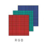
Color images have three RGB color channels, which can be represented by two-dimensional arrays. For example, a 160x60 color picture can be represented by an array of 160 * 60 * 3.
Convolution operation can extract image features. The convolution kernel is used to scan the pixel matrix of each layer continuously according to the step size. The value scanned each time is multiplied by the number of corresponding positions in the convolution kernel, and then added and summed. The obtained value will generate a new matrix. The size of convolution kernel is usually 3x3 and 5x5, but the training effect of the former will be better. Each value in the convolution kernel is the weight (neuron parameters in the process of training the model). It starts to set random initial values. In the process of training, the network will continuously update these parameter values through backward propagation until the best parameter value is found. This optimal parameter value is evaluated by the loss loss function.
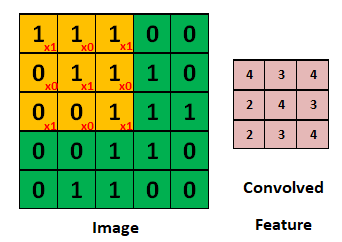
Image is a 5x5 size image that needs to be convoluted, and the convoluted feature is the feature image obtained after convolution; The Yellow matrix is a 3x3 Filter. In the process of convolution, the Filter is multiplied by the corresponding position of the image and then added to obtain the value of the central position at this time, and then fill in the first row and first column of the involved feature feature graph. Then move one of them (stripe = 1) and continue to convolute with the next position until the 3x 3x3x1 matrix is finally obtained.
Calculation of the width and height of the feature graph of the convoluted feature: the matrix dimension of the convoluted feature = (Image matrix dimension - Filter matrix dimension + 2xpad)/2+1.
Width= (5-3+2x0)/1+1,Height=(5-3+2x0)/1+1
Padding operation can better extract boundary features. In the process of image convolution, the values in the middle are easy to be extracted many times, but the feature extraction times of boundary values are relatively few. In order to better extract boundary features, a layer of 0 can be added around the original data matrix, which is the padding operation.
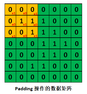
If the above example is padded, the image size will not change after convolution, such as the image size of 5x5.
Padding=1 becomes 7x7, and then convolute with 3x3 Filter, then the width and height after convolution is (7-3+2x1) / 1 + 1 = 7
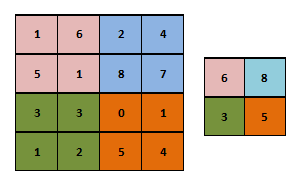
Pooling can be used for dimensionality reduction, including maximum pooling and average pooling, of which Max pooling is the most commonly used.
After convolution operation, the feature information extracted by us will have similar feature information in adjacent areas, which can be replaced by each other. If all these feature information are retained, there will be information redundancy and increase the difficulty of calculation. The spatial size of data can be reduced through the pooling layer, the number of parameters and the amount of calculation will decrease accordingly, and the over fitting is also controlled to a certain extent.
Max Pooling means that the maximum pixel value in the corresponding area of Filter replaces the pixel value. Its function is to reduce the dimension. The filters used in pooling are 2x2, so the image size obtained after pooling is 1 / 2 of the original size.
Flatten can turn the pooled data into a one-dimensional vector to facilitate input to the fully connected network.
The full connection layer is each node of layer n. during calculation, the input of the activation function is the weight of all nodes of layer n-1.
Dropout can discard the neurons in the network according to a certain proportion to prevent over fitting of the model in the training process.
Convolutional neural network VGG16 detailed explanation

As can be seen from the above figure, VGG16 has a total of five convolutions. Each convolution is followed by the maximum pooling layer. The last few layers use three full connection layers, and finally one softmax. The input of the network is a 224x224 size image, and the output is the image classification result.
VGG is analyzed in detail. Firstly, VGG is based on Alex net network. On this basis, more in-depth research on the depth and width of deep neural network is done. The industry generally believes that deeper networks have stronger expression ability than shallow networks, can depict and display better, and complete more complex tasks, but deeper networks mean more parameters and more difficult training. In order to better explore the impact of depth on the network, we must solve the problem of parameter quantity.
In VGG, the LRN layer of Alexnet is cancelled and 3x3 convolution kernel is adopted, which has less parameters than that of Alexnet with 7x7 convolution kernel. The pool core becomes smaller. The pool core of VGG is 2x2, and the stripe is 2. The pool core of Alex net is 3X3, and the step size is 2.
Due to the characteristics of convolution neural network, 3x3 convolution kernel is enough to capture the changes of horizontal, vertical and diagonal pixels. The use of large convolution kernel will lead to an explosion of parameters. Needless to say, some parts of the image will be convoluted many times, which may bring difficulties to feature extraction. Therefore, 3x3 convolution is widely used in VGG.
In the last three layers of VGG network, the parameters of the full connection layer account for a large part of the overall parameters of VGG. In order to reduce the amount of parameters, the full connection networks of the latter layers are replaced by global average pooling and convolution operations, but global average pooling also has great advantages.
VGG is a good feature extractor, and its trained model is often used to do other things, such as calculating perceptual loss (in style migration and super-resolution tasks). Although Resnet and perception networks have high accuracy and simpler network structure, VGG has always been a good network in feature extraction, so, When you don't perform well on some tasks such as Resnet or Inception, you might as well try VGG, which may have unexpected results.
VGG is not much improved for Alexnet. The main improvement is the use of small convolution kernel. The network is a piecewise convolution network. It is excessive through maxpooling, and the network is deeper and wider.
After understanding the basic concepts, we can now enter the network model of VGG16.
1. From input to Conv_1: Since 224 is not easy to calculate, use the input picture size of 300x300x3 for example:
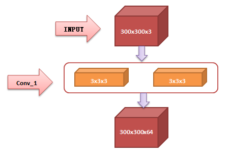
The first two yellow convolution layers are the first layer (Conv1_1) and the second layer (Conv1_2) among the sixteen layers of VGG16 network structure, which are collectively called Conv_1. 3x3x3 convolution core (Filter). The image obtained by convolution core is 298x298x1 (padding is not performed here, and the step size is 1), but after filling a circle of matrix, the result is 300x300x1. There are 64 convolution cores in this layer, so the original 300x300x1 becomes 300x300x64.
2. From Conv_1 to Conv_2. Transition between:

The Filter used by Pooling is 2x2x64 and the step size is 2. The obtained matrix dimension is just half of the original dimension. The third dimension 64 does not change because it refers to the number of filters.
3.Conv_2 to Conv_3:
The picture with Input of 300x300x3 passes through the first layer (which consists of 64 convolution cores). Then it becomes 150x150x64. The second layer consists of 128 convolution kernels. From the above law, the second layer can be deduced to obtain 75x75x128.
4.Conv_3 to Conv_4:
There are 256 convolution kernels in the second layer. From the above law, we can deduce the second layer and get 75x75x256.
VGG16 network model parameter chart
| Layer (type) Output Shape Param # |
| conv2d_1 (Conv2D) (None, 224, 224, 64) 1792 |
| conv2d_2 (Conv2D) (None, 224, 224, 64) 36928 |
| max_pooling2d_1 (MaxPooling2 (None, 112, 112, 64) 0 |
| conv2d_3 (Conv2D) (None, 112, 112, 128) 73856 |
| conv2d_4 (Conv2D) (None, 112, 112, 128) 147584 |
| max_pooling2d_2 (MaxPooling2 (None, 56, 56, 128) 0 |
| conv2d_5 (Conv2D) (None, 56, 56, 256) 295168 |
| conv2d_6 (Conv2D) (None, 56, 56, 256) 590080 |
| conv2d_7 (Conv2D) (None, 56, 56, 256) 590080 |
| max_pooling2d_3 (MaxPooling2 (None, 28, 28, 256) 0 |
| conv2d_8 (Conv2D) (None, 28, 28, 512) 1180160 |
| conv2d_9 (Conv2D) (None, 28, 28, 512) 2359808 |
| conv2d_10 (Conv2D) (None, 28, 28, 512) 2359808 |
| max_pooling2d_4 (MaxPooling2 (None, 14, 14, 512) 0 |
| conv2d_11 (Conv2D) (None, 14, 14, 512) 2359808 |
| conv2d_12 (Conv2D) (None, 14, 14, 512) 2359808 |
| conv2d_13 (Conv2D) (None, 14, 14, 512) 2359808 |
| max_pooling2d_5 (MaxPooling2 (None, 7, 7, 512) 0 |
| flatten_1 (Flatten) (None, 25088) 0 |
| dense_1 (Dense) (None, 4096) 102764544 |
| dropout_1 (Dropout) (None, 4096) 0 |
| dense_2 (Dense) (None, 4096) 16781312 |
| dropout_2 (Dropout) (None, 4096) 0 |
| dense_3 (Dense) (None, 1000) 4097000 |
| Total params: 138,357,544 |
| Trainable params: 138,357,544 |
| Non-trainable params: 0 |
On data processing and analysis
Basic concepts
Training set: as the name suggests, it refers to the sample set used for training, which is mainly used to train the parameters in the neural network.
Validation set: literally, it refers to the sample set used to verify the performance of the model. After different neural networks are trained on the training set, the performance of each model is compared and judged by the verification set Different models here mainly refer to neural networks corresponding to different superparameters, or neural networks with completely different structures.
Test set: for the trained neural network, the test set is used to objectively evaluate the performance of the neural network.

Data enhancement: data enhancement, also known as data amplification, enables limited data to produce value equivalent to more data without adding substantial data. The essence of data enhancement is to obtain better diversity. Data enhancement can be divided into supervised data enhancement and unsupervised data enhancement. This experiment uses the supervised training method, so it focuses on the introduction of supervised data enhancement.
Supervised data enhancement can be divided into single sample data enhancement and multi sample data enhancement. Supervised data enhancement, that is, using preset data transformation rules to expand data on the basis of existing data, including single sample data enhancement and multi sample data enhancement, in which single sample also includes geometric operation and color transformation. Geometric operations include flipping, rotation, clipping, deformation, scaling and other operations. Color transformation includes noise, blur, color transformation, erasure, filling and other operations.
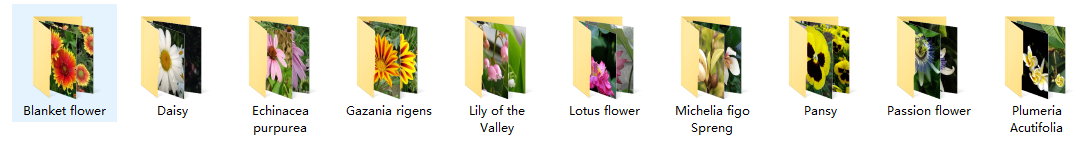
Here, we found the data of 10 kinds of flowers on the Internet, classified the data and put it in various folders. The file name is the label of flowers, and then unified the picture size to 100 * 100. The data set is divided into training set, validation set and test set. There are 4076 training sets, 811 verification sets and 157 test sets respectively. Data enhancement is required for the training set, but not for the verification set and test set.
Fine tuning model: the widely used model reuse method is fine tuning, which is complementary to feature extraction. For the frozen model base used for feature extraction, fine tuning refers to "thawing" the top layers. And the thawed layers are jointly trained with the newly added part (in this case, the fully connected classifier). Fine tuning is called because it only slightly adjusts the more abstract representations in the reused model to make them more relevant to the problem at hand.
The convolution basis of VGG16 is frozen so that a randomly initialized classifier can be trained on it. Similarly, only after the above classifier and training are completed, can the top layers of convolution basis be fine tuned. If the classifier is not well trained, the error signal through the propagation network during training will be particularly large, and the representations learned before the fine-tuning layers will be destroyed.
3.2 data preprocessing
1. File Renamer Turbo
# -*- coding:utf8 -*-
import os
class BatchRename():
    '''
    Batch rename picture files in folders
    '''
    def __init__(self):
        self.path = r'E:\flower_10\Blanket flower'
        self.label = ' Blanket flower_'
    def rename(self):
        filelist = os.listdir(self.path)
        total_num = len(filelist) #Get the number of all files in the folder
        i = 0  #Indicates that the file naming starts with 1
        for item in filelist:
            if item.endswith(('.jpeg','png','jpg')):
                src = os.path.join(os.path.abspath(self.path), item)
                dst = os.path.join(os.path.abspath(self.path),
str(self.label)+str(i) + '.jpg')
                try:
                    os.rename(src, dst)
                    print ('converting %s to %s ...' % (src, dst))
                    i = i + 1
                except:
                    continue
        print ('total %d to rename & converted %d jpgs' % (total_num, i))
if __name__ == '__main__':
    demo = BatchRename()
    demo.rename()
2. Use the existing data enhancement method ImageDataGenerator of keras
from keras.preprocessing.image import ImageDataGenerator
train_datagen = ImageDataGenerator(
                    rescale=1./255,
                    rotation_range=25,
                    width_shift_range=0.1,
                    height_shift_range=0.1,
                    shear_range=0.1,
                    zoom_range=0.1,
                    horizontal_flip=True,
                    vertical_flip = True,
                    fill_mode = 'nearest')
3.3} VGG16 fine tuning model training and testing
The steps to fine tune the network are as follows:
1. Add a custom network to the trained base network
2. Frozen base network
3. Added parts of training
4. Some layers of thaw based network
The first three steps have been completed when doing feature extraction. Continue with step 4: thaw the conv first_ Base then freezes some of its layers.
conv_base.trainable = True
set_trainable = False
for layer in conv_base.layers:
    if layer.name == 'block5_conv1':
        set_trainable = True
    if set_trainable:
        layer.trainable = True
    else:
        layer.trainable = False
We'll fine tune the last three convolutions, that is, know block4_ All layers of the pool should be frozen, while block5_conv1,block_conv2 and block_conv3 layer 3 should be trainable.
Why not fine tune more layers? Why not fine tune the entire convolution basis? Of course you can, but there are a few points to consider:
1. The layer closer to the bottom of the convolution base encodes more general reusable features, while the layer closer to the top encodes more specialized features.
2. Fine tuning the layer closer to the bottom will get less return.
3. The more training parameters, the greater the risk of over fitting. The convolution basis has 15 million parameters, so it is risky to train so many parameters on small data sets.
4. Freeze all layers up to a layer.
- Fine tuning model training
# Fine tuning model
model.compile(loss='categorical_crossentropy',optimizer=optimizers.RMSprop(lr=1e-5),metrics=['acc'])
history = model.fit_generator(train_generator,steps_per_epoch=25,epochs=100,validation_data=validation_generator, validation_steps=32,shuffle=True)
# Accuracy of test set
test_datagen = test_datagen.flow_from_directory(
    test_dir,
    target_size=(100,100),
    batch_size=30,
    class_mode='categorical'
)
test_loss,test_acc = model.evaluate_generator(test_datagen,steps=30)
print('test acc:',test_acc)
# Good practice, save model
model.save(r'.\model\flower.h5')
- Use matplotlib to draw loss and acc result graphs
# Draw the loss function curve and accuracy curve in the training process
import matplotlib.pyplot as plt
acc=history.history['acc']
val_acc=history.history['val_acc']
loss=history.history['loss']
val_loss=history.history['val_loss']
epochs=range(1,len(acc)+1)
plt.plot(epochs,acc,'bo',label='Training acc')
plt.plot(epochs,val_acc,'b',label='Validation acc')
plt.title('Training and Validation acc')
plt.legend()
plt.figure()
plt.plot(epochs,loss,'bo',label='Training loss')
plt.plot(epochs,val_loss,'b',label='Validation loss')
plt.title('Trainig and Validation loss')
plt.legend()
plt.show()
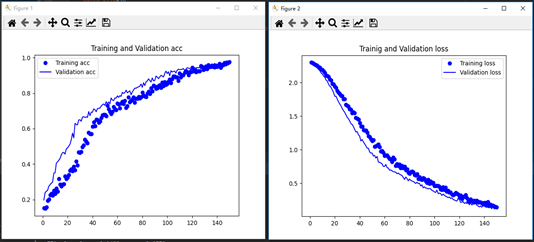
Training and Validation acc/loss diagram
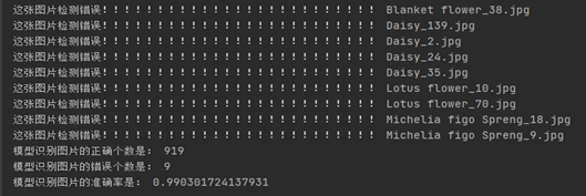
- Error analysis of fine tuning model
Formula: error rate of the model = number of different predicted categories and known category labels / total predicted labels
import os
flower_lst = ['Blanket flower', 'Daisy', 'Echinacea purpurea', 'Gazania rigens', 'Lily of the Valley', 'Lotus flower', 'Michelia figo Spreng', 'Pansy', 'Passion flower', 'Plumeria Acutifolia']
import numpy as np
from keras.models import load_model
model=load_model(r".\CNN_Flower\WY_6.h5")
from keras.preprocessing.image import ImageDataGenerator
test_datagen = ImageDataGenerator(rescale=1./255)
path = r'.\dir'
flower_path=r".\test"
test_generator = test_datagen.flow_from_directory(path, target_size=(100, 100),batch_size=1,class_mode='categorical', shuffle=False,)
#Establish the relationship between prediction results and file names
filenames = test_generator.filenames
length = len(os.listdir(flower_path))
test_generator.reset()
pred = model.predict_generator(test_generator, verbose=1, steps=length)
predicted_class_indices = np.argmax(pred, axis=1)
correct=0
error=0
filenames = test_generator.filenames
for i in range(len(filenames)):
    if filenames[i].split("\\")[1].split("_")[0]==
		flower_lst[predicted_class_indices[i]]:
        correct=correct+1
    else:
        error=error+1
        print("This picture is detected incorrectly!!!!!!!", filenames[i].split("\\")[1])
print("The correct number of model recognition pictures is:",correct)
print("The number of errors in model recognition pictures is:",error)
print("The accuracy of model recognition image is:",correct/(correct+error))
Fine tune the model and increase the test sample picture
- Fine tuning model prediction picture label
from keras.models import load_model
import cv2
import imageio
from keras.models import Model, load_model
from keras.applications.imagenet_utils import preprocess_input
from keras.preprocessing import image
import numpy as np
import matplotlib.pyplot as plt
test_model=load_model(r".\CNN_Flower\model.h5")
import os
import numpy as np
all_path = r".\test"
lst = os.listdir(all_path)
for file_path in os.listdir(all_path):
    path = os.path.join(all_path,lst[label])
    for file_name in os.listdir(path)[0:len(os.listdir(path))]:
        img_path = os.path.join(path,file_name)
        src=cv2.imread(img_path)
        src=cv2.resize(src,(100,100))
        src=src.reshape((1,100,100,3))
        src=src.astype("int32")
        src=src/255
        predict = test_model.predict(src)
        predict = np.argmax(predict, axis=1)
        print(predict)
Interface design
First enter cmd, and then execute the commands PIP install pyqt5 and pip install pyqt5} pyqt5 tools. Then design the layout and space on this canvas, as shown in the figure below. After the design is completed, convert it to py file.
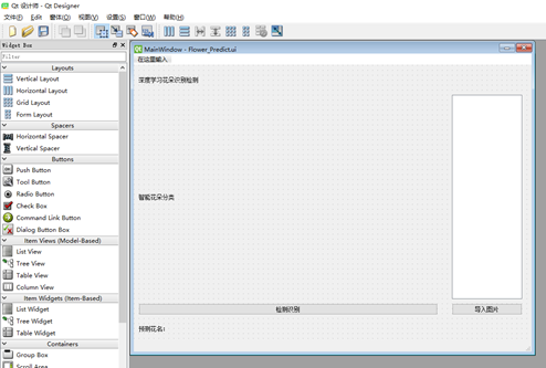
Next, you can add and bind functions in this py file.
- file open
def open_img(self):
    global imgName
    imgName, imgType = QtWidgets.QFileDialog.getOpenFileNames(self.pushButton_2, "Multi file selection","./test", "All documents (*);;text file (*.txt)")
    if len(self.imglist) == 0:
        self.imglist = imgName
    else:
        for i in range(len(imgName)):
            self.imglist.append(imgName[i])
    from functools import reduce
    img_func = lambda x, y: x if y in x else x + [y]
    self.imglist = reduce(img_func, [[], ] + self.imglist)
    slm = QStringListModel()
    slm.setStringList(self.imglist)
    self.listView.setModel(slm)
    print("HEHEDA")
- Click event
def clicked(self, qModelIndex):
    global path
    jpg = QtGui.QPixmap(self.imglist[qModelIndex.row()]).scaled(self.label.width(), self.label.height())
    self.label.setPixmap(jpg)
    path = self.imglist[qModelIndex.row()]
    self.pic_exists = 1
    self.predict_request = 1
    real_imglabel = path.split('/')
    real_imglabel = "Real flower name:" + str(real_imglabel[-2])
    self.label_4.setText(real_imglabel)
    predict_flower_name = 'Predicted flower name:'
    self.label_5.setText(predict_flower_name)
- test result
def predict_request_add(self):
    if self.predict_request<1:
        self.predict_request = self.predict_request + 1
def predict(self):
    if self.pic_exists and self.predict_request:
        print("The model test officially began")
        import os
        import cv2
        import numpy as np
        img_path = path
        src = cv2.imread(img_path)
        src = cv2.resize(src, (100, 100))
        src = src.reshape((1, 100, 100, 3))
        src = src.astype("int32")
        src = src / 255
        predict = self.model.predict(src)
        predict = np.argmax(predict, axis=1)
        print("The prediction result is:")
        print(self.img_label[predict[0]])
        predict_flower_name = self.img_label[predict[0]]
        predict_flower_name = 'Predicted flower name:' + predict_flower_name
        self.label_5.setText(predict_flower_name)
        print("In execution....")
        self.predict_request = 0
    else:
        print("Please select a picture!!!!!")
    print("end of execution")
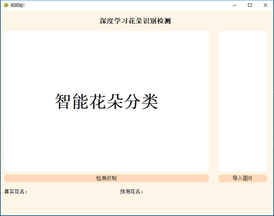
- Initialization interface display

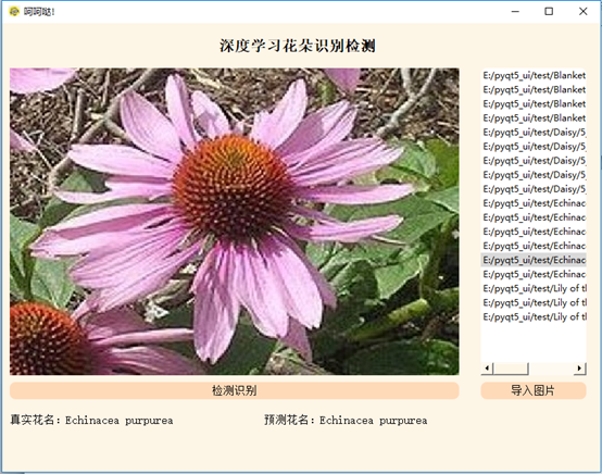
- UI interface prediction picture effect display


I love learning, hehe Da ~ if you think the article is great and helpful to you, you can praise + collect + pay attention~
If the article is incorrect, please exchange and correct it. I will consult ~o (> ω<) o
I will update the articles regularly and continue to provide you with high-quality articles
Later, ha ha Da will send the whole project to Github and other platforms for your reference and learning!!!
