TabNet released by Google is a neural network for tabular data. It realizes instance wise feature selection through sequential attention mechanism similar to additive model, and realizes self-supervised learning through encoder decoder framework.

Table data is the most commonly used data type in daily life. For example, credit card fraud detection: we extract transaction, identity, product and network attributes (and put them into a large feature table, which can be easily used by different machine learning models for training and reasoning. Decision tree based models (such as random forest or XGBoost) are the preferred algorithms for processing table data because of their performance Interpretability, training speed and robustness are the best at present.

However, neural networks are considered to be the most advanced in many fields, and perform particularly well on large data sets with the least feature engineering. Many of our customers have a large number of transactions, and deep learning is a potential way to improve the performance of the model in fraud detection.

In this article, we will deeply study the neural network architecture called TabNet (Arik & Pfister (2019)), which is designed to interpret and work well with tabular data. After explaining the key building blocks and ideas behind it, you will learn how to implement it in TensorFlow and how to apply it to fraud detection data sets. If you use pytoch, you don't have to worry. TabNet has the implementation of various deep learning frameworks.

TabNet

TabNet uses the idea of Sequential Attention to simulate the behavior of decision tree. In short, it can be regarded as a multi-step neural network, and two key operations are applied in each step:

• The attention transformer selects the most important features for processing in the next step
• Use Feature Transformer to process features into more useful representations

Finally, the model uses the output of Feature Transformer for prediction later. TabNet uses both attention and Feature Transformers to simulate the decision-making process of tree based model. For example, the following prediction of adult census income data sets, the model can select and process the most useful features for the task at hand, so as to improve interpretability and learning ability.

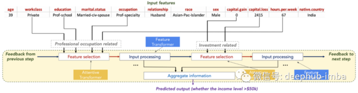
The key building blocks of attention and Feature Transformer are the so-called Feature Blocks, so let's explore them first.

Feature Block

Feature Block consists of sequential application of full connection (FC) or dense layer and batch normalization (BN). In addition, for the Feature Transformer, the output is transferred through the GLU activation layer.

The main function of GLU (as opposed to sigmoid gate) is to allow hidden units to propagate deeper into the model and prevent gradient explosion or disappearance.

def glu(x, n_units=None):
    """Generalized linear unit nonlinear activation."""
    return x[:, :n_units] * tf.nn.sigmoid(x[:, n_units:])

In the original paper, ghost batch normalization is used in the training process to improve the convergence speed. If you are interested, you can search for the relevant introduction, but in this article, we will use the default BN layer.

class FeatureBlock(tf.keras.Model):
    """
    Implementation of a FL->BN->GLU block
    """
    def __init__(
        self,
        feature_dim,
        apply_glu = True,
        bn_momentum = 0.9,
        fc = None,
        epsilon = 1e-5,
    ):
        super(FeatureBlock, self).__init__()
        self.apply_gpu = apply_glu
        self.feature_dim = feature_dim
        units = feature_dim * 2 if apply_glu else feature_dim # desired dimension gets multiplied by 2
                                                              # because GLU activation halves it

        self.fc = tf.keras.layers.Dense(units, use_bias=False) if fc is None else fc # shared layers can get re-used
        self.bn = tf.keras.layers.BatchNormalization(momentum=bn_momentum, epsilon=epsilon)

    def call(self, x, training = None):
        x = self.fc(x) # inputs passes through the FC layer
        x = self.bn(x, training=training) # FC layer output gets passed through the BN
        if self.apply_gpu: 
            return glu(x, self.feature_dim) # GLU activation applied to BN output
        return x

Feature Transformer

Feature Transformer (FT) is a collection of feature blocks that are applied sequentially. In this paper, a feature transformer is composed of two shared blocks (i.e. step reuse weight) and two step dependent blocks. Shared weights reduce the number of parameters in the model and provide better generalization.

The following describes how to use the Feature Block in the previous section to build the Feature Transformer.

class FeatureTransformer(tf.keras.Model):
    def __init__(
        self,
        feature_dim,
        fcs = [],
        n_total = 4,
        n_shared = 2,
        bn_momentum = 0.9,
    ):
        super(FeatureTransformer, self).__init__()
        self.n_total, self.n_shared = n_total, n_shared

        kwrgs = {
            "feature_dim": feature_dim,
            "bn_momentum": bn_momentum,
        }

        # build blocks
        self.blocks = []
        for n in range(n_total):
            # some shared blocks
            if fcs and n < len(fcs):
                self.blocks.append(FeatureBlock(**kwrgs, fc=fcs[n])) # Building shared blocks by providing FC layers
            # build new blocks
            else:
                self.blocks.append(FeatureBlock(**kwrgs)) # Step dependent blocks without the shared FC layers

    def call(self, x, training = None):
        # input passes through the first block
        x = self.blocks[0](x, training=training) 
        # for the remaining blocks
        for n in range(1, self.n_total):
            # output from previous block gets multiplied by sqrt(0.5) and output of this block gets added
            x = x * tf.sqrt(0.5) + self.blocks[n](x, training=training) 
        return x

    @property
    def shared_fcs(self):
        return [self.blocks[i].fc for i in range(self.n_shared)]

Attentive Transformer

The attention transformer (at) is responsible for feature selection at each step. Feature selection is accomplished by applying sparsemax activation (not GLU) and taking into account a priori proportions. A priori scaling allows us to control the frequency of a feature selected by the model and controlled by the frequency it used in the previous steps (described in detail later).

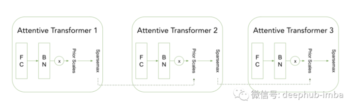
The Transformer in the previous step provides the scale information of the features in the previous step, which is equivalent to telling which features are used in the previous step. Similar to the Feature Transformer, the attention Transformer can be integrated into a larger architecture as a TensorFlow model.

class AttentiveTransformer(tf.keras.Model):
    def __init__(self, feature_dim):
        super(AttentiveTransformer, self).__init__()
        self.block = FeatureBlock(
            feature_dim,
            apply_glu=False, # sparsemax instead of glu
        )

    def call(self, x, prior_scales, training=None):
        # Pass input trhough a FC-BN block
        x = self.block(x, training=training)
        # Pass the output through sparsemax activation
        return sparsemax(x * prior_scales)

Because Feature and Transformer blocks can become very parameter dependent, TabNet uses some mechanisms to control complexity and prevent overfitting.

Regularization

Previous feature scale calculation

A priori ratio (P) allows us to control the frequency of model selection features. Use previous Attentive Transformer activation and relaxation factors( γ) Parameter calculation a priori scale (P). This is the formula proposed in the paper.

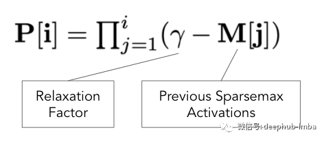
This equation shows how the a priori ratio (P) is updated. Intuitively, if a feature is used in the previous steps, the model will pay more attention to the remaining features to reduce over fitting.

For example, when γ= At 1, features with larger activation (e.g. 0.9) will have a smaller a priori scale (1-0.9 = 0.1). A small a priori scale ensures that the feature is not selected in the current step.

Sparse regularization

By super parameter λ The scaled activation entropy will be added to the overall model loss. Sparse regularization of the loss in this way can make the attention mask more sparse.

def sparse_loss(at_mask):
    loss = tf.reduce_mean(
        tf.reduce_sum(tf.multiply(-at_mask, tf.math.log(at_mask + 1e-15)),
                      axis=1)
    )
    
    return loss

not_sparse_mask = np.array([[0.4, 0.5, 0.05, 0.05],
                      [0.2, 0.2, 0.5, 0.1]])

sparse_mask = np.array([[0.0, 0.0, 0.7, 0.3],
                      [0.0, 0.0, 1, 0.0]])

print('Loss for non-sparse attention mask:', sparse_loss(not_sparse_mask).numpy())
print('Loss for sparse attention mask:', sparse_loss(sparse_mask).numpy())

# Loss for non-sparse attention mask: 1.1166351874690217
# Loss for sparse attention mask: 0.3054321510274452

Now that all the components of TabNet have been introduced, let's see how to use these components to build the TabNet model.

TabNet architecture

Put them together, the main idea of TabNet is to apply Feature and attention transformers components in order, so that the model can simulate the generation process of decision tree. The attention transformer performs Feature selection, while the Feature Transformer performs transformations that allow the model to learn complex patterns in the data. You can see a chart below that summarizes the data flow of the 2-step TabNet model.

First, the initial input feature is passed through the Feature Transformer to obtain the initial feature representation. The output of this Feature Transformer will be used as the input of the attention transformer. The attention transformer selects a feature subset to pass to the next step. There will be a super parameter to set the number of times this step is repeated.

The model generates the final prediction by using the Feature Transformer output of each decision step. In addition, at each step, pay attention to the mask to understand which features are used for prediction. These masks can be used to obtain local feature importance and global importance.

The above is the complete architecture of TabNet. Let's see how to train this model on Kaggle's fraud detection sample data set.

Fraud detection using TabNet

The data set and code used below can be found in the connection we provided at the end.

data

The training data set is very large, with about 590k pieces of data, and each data contains 420 features. The preprocessing performed is very basic because this is not the goal of this article:

• Delete non information columns
• Missing value fill
• Coding classification variable
• Time based training / verification split

Hyperparametric tuning

TabNet (like any neural network) is very sensitive to super parameters, so adjustment is very important to obtain a good model. The following are the variables (and recommended ranges) that we found to have the greatest impact on model performance:

1. Feature dimension / output dimension: from 32 to 512 (we usually set these parameters to equal values, because this is also recommended in the paper)
2. Steps: from 2 (simple model) to 9 (very complex model), which is the super parameter in the architecture
3. Relaxation factor: from 1 (force feature only in step 1) to 3 (relax constraint)
4. Sparse coefficient: from 0 (no regularization) to 0.1 (strong regularization)

A simple HP tuning example is also given in the code provided at the end of the paper.

Training and evaluation

Similar to other models, training TabNet can further improve the performance by experimenting with learning rate scheduling and attenuation.

# Params after 1 hour of tuning
tabnet = TabNet(num_features = train_X_transformed.shape[1],
                output_dim = 128,
                feature_dim = 128,
                n_step = 2, 
                relaxation_factor= 2.2,
                sparsity_coefficient=2.37e-07,
                n_shared = 2,
                bn_momentum = 0.9245)

# Early stopping based on validation loss    
cbs = [tf.keras.callbacks.EarlyStopping(
        monitor="val_loss", patience=30, restore_best_weights=True
    )]

# Optimiser 
optimizer = tf.keras.optimizers.Adam(learning_rate=0.01, clipnorm=10)

# Second loss in None because we also output the importances
loss = [tf.keras.losses.CategoricalCrossentropy(from_logits=False), None]

# Compile the model
tabnet.compile(optimizer,
               loss=loss)

# Train the model
tabnet.fit(train_ds, 
           epochs=1000, 
           validation_data=val_ds,
           callbacks=cbs,
           verbose=1,
           class_weight={
             0:1,
             1: 10
           })

ROC and PR AUC scores are usually used to evaluate the model (because the target is unbalanced), so here are the indicators on the validation set of the model.

Test ROC AUC 0.8505
Test PR AUC 0.464

The result is OK, but it's not very good, but the purpose of this paper is not to get the ranking. Our purpose is how to build and train the TabNet model.

summary

This paper introduces the architecture of TabNet and how it uses attention and Feature Transformers to predict. TabNet has a lot of content that we haven't covered (such as attention mask and self-monitoring pre training), so if you want to further explore this model, please read the following resources:

Author: Anton Rubert