This article is excerpted from the fourth chapter of Keras deep learning: introduction, actual combat and advanced.

What is EBImage

EBImage is an extension package of R. it provides general functions for reading, writing, processing and analyzing images, which is very easy to use. The EBImage package is installed in Bioconductor through the following command.

install.packages("BiocManager")
BiocManager::install("EBImage")

After EBImage is installed, it can be loaded into R through the following command.

library("EBImage")

1. Image reading and saving

The basic functions of EBImage include image reading, display and writing. Use the readImage() function to read the image. The parameter files in the function indicates the file name or URL to be read, and the parameter type indicates the image file format to be read. At present, jpeg, png and tiff image file formats are supported.
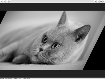
First, we will load a gray image in jpg file into R. We can visualize the image just loaded through the display() function

> img <- readImage('../images/cat.jpg')
> display(img ,method = 'browser')

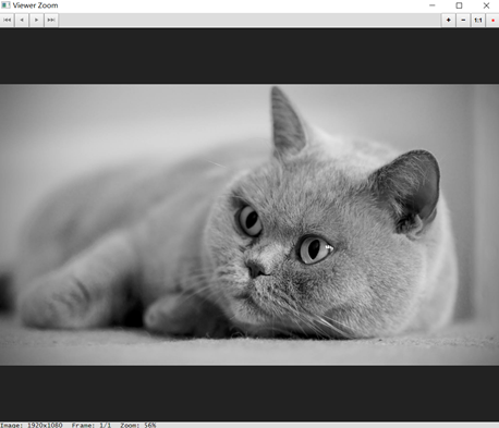
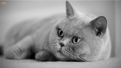
When the parameter method of the display() function is "browser", the image will be opened in the default Web browser after running the command in R, and the interactive image will be opened in the View window after running the command in RStudio. Use the mouse or keyboard shortcuts to zoom in or out, pan, or cycle through multiple images. When the parameter method is "raster", the static image will be drawn on the current device. We can also use R's low-level drawing function to add other elements to the image. Running the following program code will add a text label to the image

> display(img,method = 'raster')
> text(x = 20,y = 20,label = 'cat',adj = c(0,1),col = 'orange',cex = 2)

The above example reads in black-and-white images (or gray images), and the readImage() and display() functions can also easily read in color photos.

> imgcol <- readImage('../images/cat-color.jpg')
> display(imgcol,method = 'raster')

2. Color management

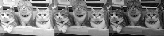
The colorMode() function can be used to access and change this property to modify the rendering mode of the image. In the next example, we change the mode of a color image to Grayscale, then the image will no longer display a single color image, but will be converted to a three frame gray image, corresponding to red, green and blue channels respectively. The colorMode() function only changes the way the EBImage renders the image, not the content of the image. Run the following program code to render a color image into a gray image with 3 frames (red channel, green channel, blue channel).

> colorMode(imgcol) <- Grayscale
> display(imgcol,method = 'raster',all = TRUE,nx = 3)

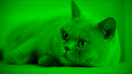
We can use the more flexible channel () function to convert the color space, convert the gray image into the color image, and extract the color channel from the color image. Unlike the colorMode() function, the channel() function can also change the pixel intensity value of the image. asred, asgreen and asblue conversion modes can convert gray images or arrays into color images with specified tones. At this time, the graphics data will also change from two-dimensional to three-dimensional.

> img_asgreen <- channel(img,'asgreen')
> dim(img)
[1] 1920 1080
> dim(img_asgreen)
[1] 1920 1080    3

3. Image processing

As a numeric array, you can easily manipulate images using any arithmetic operator of R. For example, we can generate a negative image by simply subtracting the image data from its maximum value.

> img_neg <- max(img) - img
> img_comb <- combine(img,img_neg) TRUE)

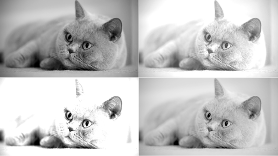
We can also add to increase the brightness of the image, adjust the contrast by multiplication, and apply gamma correction by exponentiation.

> img_comb1 <- combine(
+   img,
+   img + 0.3,
+   img * 2,
+   img ^ 0.5
+ )
> display(img_comb1,method = 'raster',all=TRUE)

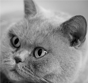
We can use the subset selection method of the standard matrix to cut the Image. For example, we select some data of Image class to draw the head of cat

> img_crop <- img[800:1700, 100:950]
> plot(img_crop)

4. Spatial transformation

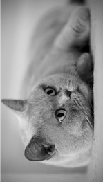
For gray images, you can use the t() function of R basic package or the transfer() function of EBImage extension package to transpose.

> img_t <- transpose(img) # Equivalent to img_ t <- t(img)
> plot(img_t)

For color images, we can't use the t() function, but need to use the transfer () function to transpose them, which can replace the image by exchanging spatial dimensions.

> t(imgcol) # report errors
Error in t.default(imgcol) : argument is not a matrix
> imgcol_t <- transpose(imgcol)
> plot(imgcol_t)

In addition to transpose, we have more about the spatial transformation of images, such as translation, rotation, reflection and scaling. The translate() function moves the image plane through the specified two-dimensional vector, cuts the pixels outside the image area, and sets the pixels entering the image area as the background. Parameter v is a vector composed of two numbers, representing the translation vector in pixels. The following code moves the image 100 pixels to the right and 50 pixels up.

> img_rotate <- rotate(img,30)
> plot(img_rotate)

Use the resize() function to scale the image. If only one of the width or height is provided, the other size will be automatically calculated and the original aspect ratio will be maintained. The following code sets the width and height of img and imgcol images to 256.

> # Resize image
> img_resize <- resize(img,w = 256,h = 256)
> imgcol_resize <- resize(imgcol,w = 256,h = 256)
> par(mfrow=c(1,2))
> plot(img_resize)
> plot(imgcol_resize)
> par(mfrow=c(1,1))

The flip() and flop() functions reflect the image around the horizontal and vertical axes, respectively.

> img_flip <- flip(img)
> img_flop <- flop(img)
> display(combine(img_flip, img_flop), 
+         all=TRUE,method = 'raster')

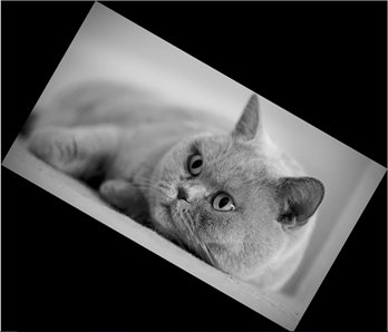
The affine() function can realize spatial linear transformation, in which the pixel coordinates (expressed by matrix px) are transformed into cbind(px, 1)%*%m.

> m <- matrix(c(1,-.5,128,0,1,0),nrow=3,ncol=2)
> img_affine <- affine(img, m)
> display(img_affine)

5. Morphological operation

Binary image is an image that contains only two groups of pixels. Its values are 0 and 1, representing background pixels and foreground pixels respectively. Such an image has to undergo several nonlinear morphological operations: erosion, expansion, opening and closing. These operations work by overlaying a mask called a structural element on the binary image in the following ways:

• Corrosion: for each foreground pixel, place a mask around it. If any pixel covered by the mask comes from the background, set it as the background.
• Swell: for each background pixel, place a mask around it. If any pixel covered by the mask comes from the foreground, set the pixel to the foreground.
  We first read in a binary image, then use markBrush() function to create a filter with the shape of diamond and the size of 3, then corrode the binary image through erode() function and expand the image through dilate() function.

> shapes <- readImage('../images/shapes.png')
> kern = makeBrush(3, shape='diamond')
> shapes_erode= erode(shapes, kern) # corrosion
> shapes_dilate = dilate(shapes, kern) # expand
> display(combine(shapes,shapes_erode, shapes_dilate), 
+         all=TRUE,method = 'raster',nx = 3)

6. Image segmentation

Image segmentation refers to the segmentation of the image, which is usually used to identify the objects in the image. Contactless connected objects can be segmented using the bwlabel() function, while the watershed() and propagate() functions can separate objects in contact with each other with more complex algorithms.
The bwlabel() function looks for each contiguous set of pixels other than the background and relabels the sets with a uniquely incremented integer. It can be called on binary images with thresholds to extract objects.

> shapes_label <- bwlabel(shapes)
> table(shapes_label)
shapes_label
 0     1     2     3     4     5     6     7     8     9    10    11    12    13    14    15 
16821   398   129   135   11   147    81   109    60    87    93    81    78   100    87    15 
> max(shapes_label)
[1] 15

shapes_ The pixel value of the label image ranges from 0 (corresponding to the background) to the number of objects it contains, and the maximum value is 15.
We use the normalize() function to normalize it in the (0,1) range, which will cause different objects to be rendered with different gray shadows

> display(normalize(shapes_label),method = 'raster') # Gray rendering

Another way to visualize segmentation is to use the colorLabels() function, which encodes objects by random arrangement of unique colors.

> display(colorLabels(shapes_label),method = 'raster') # Color rendering

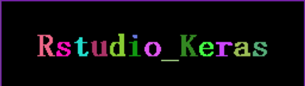
EBImage defines an object mask as a set of pixels with the same unique integer value. Usually, an image containing an object mask is the result of a segmentation function, such as bwlabel, watershed, or propagate. Objects can be deleted from these images through the rmObject() function. You can delete objects from the mask by setting the pixel value of the objects to 0. By default, after deleting objects, all remaining objects are relabeled so that the highest object ID corresponds to the number of objects in the mask. The parameter reenumerate can be used to change this behavior and retain the original object ID.
We need to bring rstudio_ '' in keras object Remove, through the following program code.

> z <- rmObjects(shapes_label,15) # Remove "_"
> display(z,method = 'raster')