Swin Transformer
Original link: https://www.cnblogs.com/dan-baishucaizi/p/14661164.html
Thesis address: https://arxiv.org/abs/2103.14030
Project address: https://github.com/microsoft/Swin-Transformer
abstract
This paper presents a new vision Transformer, called swing Transformer, which can be used as a general backbone of computer vision. The transformation of Transformer from language to vision faces great challenges. It mainly comes from the differences between the two fields. For example, the scale of visual entities changes greatly, and the pixels in the image have high resolution compared with the words in the text. In order to solve these differences, we propose a hierarchical Transformer, whose representation is calculated by shifted window. The sliding window scheme improves the efficiency by limiting the self attention calculation to non overlapping local windows and allowing cross window connections. This hierarchical architecture has the flexibility of modeling at various scales, and has linear computational complexity related to image size. These features of swing Transformer make it compatible with a wide range of visual tasks, including image classification (86.4 top-1 accuracy on ImageNet-1K) and intensive prediction tasks, such as target detection (58.7 box AP and 51.1 mask # AP on COCO test DEV) and semantic segmentation (53.5 mIoU on ADE20K val). Its performance exceeds the previous advanced level. The box AP and mask AP on COCO are + 2.7 and + 2.6 respectively, and the mask AP and + 3.2 million on ADE20K show the potential of Transformer based model as visual backbone.
1. Introduction
In the process of computer vision modeling, CNN network has achieved excellent performance, and a lot of work has been done based on CNN network in the past few years; In the NLP field, up to now, Transformer has increasingly become a baseline, which has a good performance in dealing with long-term dependence. Its great success in the field of language has prompted researchers to study its adaptability to computer vision. Recently, it has shown promising results on some tasks, especially image classification [19] and joint visual language modeling [46].
In this paper, we try to extend the applicability of Transformer so that it can be used as a general backbone of computer vision like CNN. We observed that the major challenge of transferring its high performance in the language field to the visual field can be explained by the difference between the two models. One of the differences relates to size. Different from the word tokens as the basic element processed in the language Transformer, the visual elements may be very different in scale, which is a problem of concern in tasks such as target detection [41, 52, 53]. At present, based on the Transformer method, tokens are of fixed size, which is not suitable for vision. Another major difference is that visual pixels have a higher resolution than text. For instance segmentation, we need to process and calculate at the pixel level, so the computational complexity of self attention is very high. In order to overcome this problem, we propose a general Transformer backbone: (swing Transformer), which constructs hierarchical feature mapping, and the computational complexity is linear with the image size. As shown in the figure below:
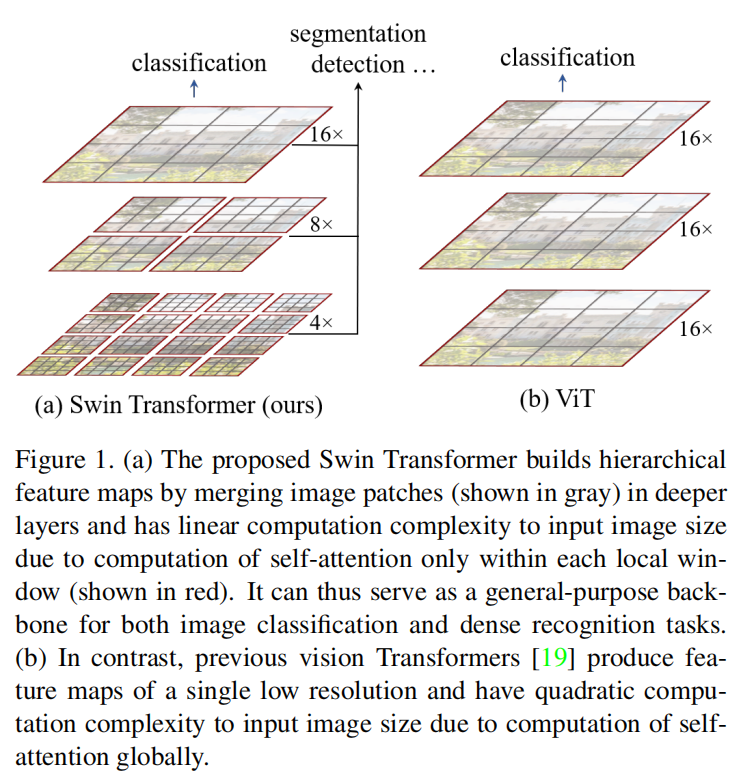
Swing Transformer constructs a hierarchical representation, starting with small pixel blocks (represented by gray) and gradually merging deeper pixel blocks. With these hierarchical feature maps, the swin Transformer model can easily use advanced technologies for intensive prediction, such as feature pyramid network (FPN) [41] or U-Net[50]. The linear computational complexity is achieved by locally calculating self attention in the non overlapping window (red contour) of the segmented image. The number of pixel blocks in each window is fixed, so the complexity is linear with the image size. This makes the swing Transformer as the backbone can adapt to various visual tasks. The former Transformer technology for vision only uses single-layer feature map and has quadratic complexity.
A key design element of swing transformer is its window partition movement between successive layers of self-interest, as shown in Figure 2.
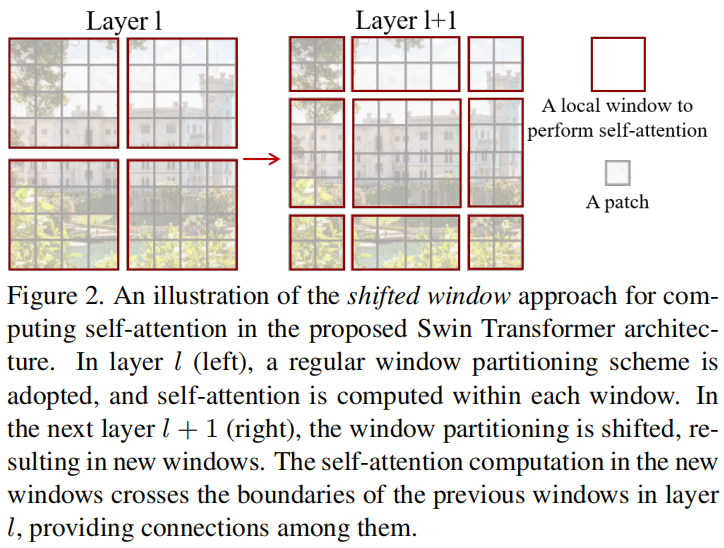
The shifted window bridges the windows of the previous layer, provides the connection between them, and significantly enhances the modeling ability (see Table 4). This strategy is also effective for latency: all query pixel blocks in a window share the same key, which is helpful for memory access in hardware. Our experiments show that the proposed moving window method has lower delay than the sliding window method, but it is similar in modeling ability.
Swing transformer achieves stronger performance: on the premise of similar latency, it is better than ResNe(X)t models and ViT / DeiT! 58.7% 58.7% box AP, 51.1% 51.1% mask AP and test data coco test dev set are realized, which is 2.7p2 higher than the previous SOTA model 7P,2.6P2.6P; mIoU value increased by 3.2, reaching 86.4% 86.4% Top-1 accuracy on ImageNet-1K.
We believe that a unified architecture across computer vision and natural language processing can benefit both fields, because it will promote the joint modeling of visual and text signals, and the modeling knowledge from the two fields can be shared more deeply. We hope that the excellent performance of swing transformer on various visual issues will promote the community to deepen this belief and encourage the unified modeling of visual and linguistic signals.
2. Related work
2.1 CNN and its variants
AlexNet ---> VGG,GoogleNet,ResNet, DenseNet, HRNet,EffificientNet.
Based on these evolutions, there are famous:
- Depth separable convolution;
- Deformation convolution;
2.2 self attention mechanism based on backbone structure
At present, scholars are keen to replace a convolution in ResNet, which is mainly based on local window optimization. They do improve the performance. However, while improving the performance, it also increases the computational complexity. We use shift windows to replace the original sliding window, which allows a more efficient implementation in general hardware.
2.3 self attention / transformers as a supplement to CNNs
See the meaning of the name: add the self attention / Transformers structure after the traditional backbone. Our work explores Transformer's adaptation to basic visual feature extraction, which is a supplement to these work.
2.4 Transformer based backbone
The most relevant work with swing Transformer is ViT and its successors. ViT's pioneering work is to directly apply a Transformer structure to image classification on non overlapping medium-sized image blocks. Compared with convolution network, it achieves an impressive tradeoff between speed and accuracy in image classification. However, ViT needs a lot of pictures to train the network. DeiT has improved the training strategy to make the required picture set smaller. Although ViT has improved in image classification, it is not suitable for high-resolution images because its complexity is the quadratic of image size. ViT model is applied to direct up sampling or deconvolution algorithms in dense visual tasks such as target detection and semantic segmentation. Our work also changed ViT to further improve its image classification task. Based on experience, we find that our swing Transformer architecture can achieve the best speed accuracy tradeoff among these image classification methods, although our work focuses on general performance rather than classification. Other researchers are also doing multi-scale resolution fusion, but its complexity is quadratic, and our complexity is linear. Our model takes into account the performance and speed of the model, and achieves a new SOTA in COCO target detection and ADE20K semantic segmentation.
3. Method
3.1 overall structure
Figure 3 gives an overview of the swing transformer architecture, illustrating the micro Version (swing-t).
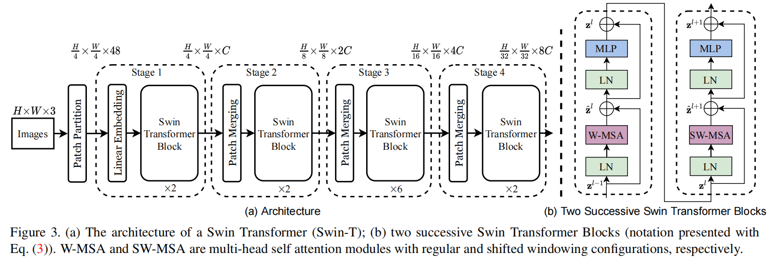
Firstly, it divides the input RGB image into non overlapping pixel blocks through a segmentation module like ViT. Each pixel block is regarded as a "token", and its feature is set as the concatenation of the RGB values of the original pixels. The pixel block we use is 4 × 4, so its characteristic dimension is 4 × four × 3=48. A linear embedding layer is applied to the original value feature and projected to any dimension (expressed as C).
In stage1, several Swin Transformer blocks operators are applied to these pixel blocks. These Transformer blocks maintain H/4 × The number of tokens of W/4, accompanied by a linear embedding layer.
In stage 2, in order to produce a hierarchical representation, the number of tokens is reduced due to the combination of pixel blocks. For the first time, the patch merging layer merged 2 × 2 pixel blocks in the field, and a linear layer is used to merge on the features of 4C. This operation is reduced by 2 × 2 = 4x tokens, and set the output dimension to 2C. After Transformer blocks are applied to feature transformation, the number of tokens becomes H/8 × W/8. This first pixel block fusion and feature transformation is called stage2. This operation generates stage3 and stage4. As shown in the figure, the number of tokens is H/16 respectively × W/16,H/32 × W/32. These stages together produce a hierarchical representation with the same characteristic image resolution as a typical convolutional network, such as VGG [51] and ResNet [29]. The results show that the architecture can easily replace the backbone in the existing methods for various visual tasks.
3.1.1 Swin Transformer block
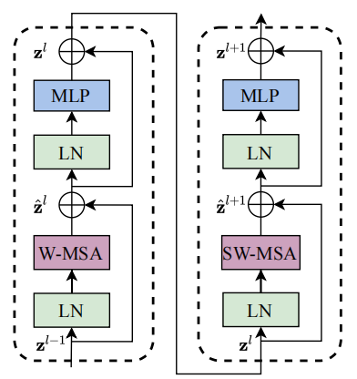
The swing transformer block uses shifted windows to replace the traditional multi head attention mechanism MSA, as shown in Figure 3(b) above. The swing transformer block is composed of MSA based shifted windows. It is surrounded by LN(LayerNorm) layer in front and LN + MLP in the back, and connected with residuals.
3.2 Shifted Window based on self attention
The standard Transformer architecture is suitable for image classification. It mainly adopts the global self attention mechanism of relative position coding, and the global computational complexity is quadratic, which is reflected in the number of tokens. This brings speed loss in many visual tasks, and shows strong adaptability in high resolution.
3.2.1 self attention of non overlapping windows
In order to calculate efficiently, we use local windows. These windows are evenly arranged and do not overlap each other. Suppose the window contains M × M pixel blocks, then global MSA is in h × The computational complexity on the image of w is:

Here, the complexity of MSA is the quadratic of hw, while M2M2 is much smaller than hwhw, so it is the primary complexity of hwhwhw.
3.2.2 shift window division of continuous blocks
The window based self attention module lacks cross window connection, which limits its modeling ability. In order to maintain the computational efficiency of non overlapping windows and introduce cross window connection, we propose a "shifted window" partition method, which alternately uses two partition configurations in continuous swing transformer blocks.
As shown in Figure 2, the first model uses the regular window partition strategy. Starting from the upper left corner, move 8 × The pixel block of 8 is divided into M × M(M=4) 2 × 2 pixel block. The strategy for the next model is shifted. Move the window divided by the upper layer: move (⌊ M/2 ⌋, ⌊ M/2 ⌋) 2 to the upper left corner × 2 pixel block. Using the moving window division method, the calculation formula of continuous swing transformer block is as follows:
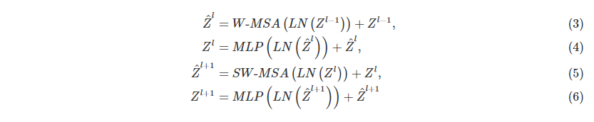
The above formula corresponds to the structure shown in Fig. 3(b).
Moving window partition strategy realizes the connection of adjacent non overlapping windows. Through experiments, we find that it is efficient for image classification, target detection and semantic segmentation! Refer to Table 4
Note: the number of pixel block features in W-MSA is consistent, but it is not consistent in SW-MSA. How to calculate this?
3.2.3 efficient batch calculation of shifted strategy
The shifted operation makes the number of pixel block patches ⌈ h/M ⌉ × ⌈ w / m ⌉ from to (⌈ h/M ⌉ + 1) × (⌈w/M⌉+1). As shown in Figure 2. And the size of some windows here is not M × M. The easiest way is to pad all windows directly to the same size. If the regular policy partition is small, such as 2 above × 2, the amount of calculation will be increased. However, we propose a batch efficient calculation method: cyclic shifting to the upper left, as shown in the figure below.
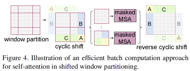
Cyclic shifting is actually non-M caused by movement × M pixel blocks are merged into M × MM × M pixel block, or you can understand that the window was moving before, but now the feature map is moving, and the part beyond the window in the upper left corner is filled in the lower right foot! After the adjustment of cyclic shifting, the size of each pixel block is actually the same. At the same time, we also realize the information fusion between different patches, and the number of patches does not change.
3.2.4 relative position offset
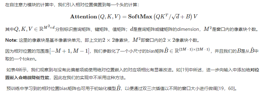
In the calculation of self attention module, we introduce the calculation of relative position offset to each head:
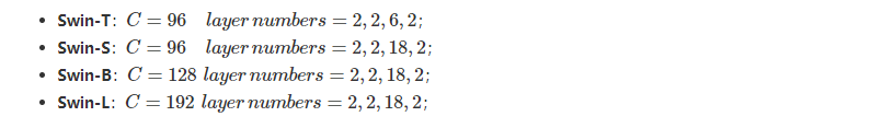
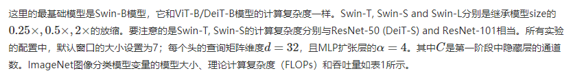
3.3 structural variants
The model architecture set by the author includes:
4. Build model interface
Interface: swing transformer models. build,build_ model
The model to be built is mainly identified here. Of course, the swing project only supports the swing project. If other configurations need to be added, they can be modified in the else section.
The main codes are:
model = SwinTransformer(img_size=config.DATA.IMG_SIZE,
                        patch_size=config.MODEL.SWIN.PATCH_SIZE,
                        in_chans=config.MODEL.SWIN.IN_CHANS,
                        num_classes=config.MODEL.NUM_CLASSES,
                        embed_dim=config.MODEL.SWIN.EMBED_DIM,
                        depths=config.MODEL.SWIN.DEPTHS,
                        num_heads=config.MODEL.SWIN.NUM_HEADS,
                        window_size=config.MODEL.SWIN.WINDOW_SIZE,
                        mlp_ratio=config.MODEL.SWIN.MLP_RATIO,
                        qkv_bias=config.MODEL.SWIN.QKV_BIAS,
                        qk_scale=config.MODEL.SWIN.QK_SCALE,
                        drop_rate=config.MODEL.DROP_RATE,
                        drop_path_rate=config.MODEL.DROP_PATH_RATE,
                        ape=config.MODEL.SWIN.APE,
                        patch_norm=config.MODEL.SWIN.PATCH_NORM,
                        use_checkpoint=config.TRAIN.USE_CHECKPOINT)
Note: here the author uses YACs Config. For details, refer to swing transformer config. py.
The parameters of SwinTransformer class are almost known by name. The specific meanings of parameters are as follows:
"""
Args:
    img_size (int | tuple(int)): Enter image size. Default 224
    patch_size (int | tuple(int)): Size of pixel block. Default: 4
    in_chans (int): Enter the number of channels for the image. Default: 3
    num_classes (int): Classification number. Default: 1000
    embed_dim (int): Dimension of pixel block coding. Default: 96
    depths (tuple(int)): each Swin Transformer Depth of layer.
    num_heads (tuple(int)): Different layers attention Number of heads.
    window_size (int): shfited window Size of, i.e M. Default: 7
    mlp_ratio (float):  MLP hidden dim reach embedding dim Ratio of. Default: 4
    qkv_bias (bool): If True, add a learnable bias to query, key, value. Default: True
    qk_scale (float): Override default qk scale of head_dim ** -0.5 if set. Default: None
    drop_rate (float): Dropout rate. Default: 0
    attn_drop_rate (float): Attention dropout rate. Default: 0
    drop_path_rate (float): Stochastic depth rate. Default: 0.1
    norm_layer (nn.Module): Normalization layer. Default: nn.LayerNorm.
    ape (bool): Add absolute position code. Default: False
    patch_norm (bool): Is it patch embedding Add after normalization. Default: True
    use_checkpoint (bool): Whether to use checkpointing to save memory. Default: False
"""5,SwinTransformer
The initialization parameters of SwinTransformer have been introduced earlier. Let's sort out the component of its model -- attribute variables.
self.num_features
This variable is passed directly without parameters and is evaluated as int (embedded_dim * 2 * * (len (depths) - 1)).
self.ape,self.absolute_pos_embed
self. Whether ape uses absolute position coding. self. absolute_ pos_ When embedded is initialized, it is an all zero tensor with shape (1, num_patches, embedded_dim) and uses trunc_normal_ The truncated normal distribution is initialized, and its standard deviation is 0.02.
Add PatchEmbed and absolute position code [absolute position code is optional], and then randomly dropout the merged feature map. According to self Layers generates forward propagation for each stage. Stage is built based on BasicLayer! Refer to 5.2.
SwinTransformer is mainly composed of PatchEmbed + layer1 + layer2 + layer3 + layer4.
The classification model is mainly connected here: ln + avgpool1d + head: NN Linear
5.1 PatchEmbed
self.patch_embed
The image is divided into non overlapping pixel blocks.
self.patch_embed = PatchEmbed(
   img_size=img_size, patch_size=patch_size, in_chans=in_chans, embed_dim=embed_dim,
   norm_layer=norm_layer if self.patch_norm else None
)
PatchEmbed is a layer based on torch implementation.
Parameters:
- img_size (int): Image size. Default: 224.
- patch_size (int): Patch token size. Default: 4.
- in_chans (int): Number of input image channels. Default: 3.
- embed_dim (int): Number of linear projection output channels. Default: 96.
- norm_layer (nn.Module, optional): Normalization layer. Default: None
Other properties:
-
self.patches_resolution: pixel block resolution, that is, the number of pixel block divisions corresponding to height and width
[img_size[0] // patch_size[0], img_size[1] // patch_size[1]]
-
self.num_patches: the number of pixel blocks, i.e. patches_resolution[0] * patches_resolution[1]
-
self.proj: convolution is used for coding, and the size of convolution kernel is patch_size and step size are also patch_size. Therefore, after the convolution process, the shape of the patch becomes 1 × one × embed_dim1 × one × embed_dim.
Forward propagation:
def forward(self, x):
    B, C, H, W = x.shape
    # FIXME look at relaxing size constraints
    assert H == self.img_size[0] and W == self.img_size[1], \
        f"Input image size ({H}*{W}) doesn't match model ({self.img_size[0]}*{self.img_size[1]})."
    x = self.proj(x).flatten(2).transpose(1, 2)  # B Ph*Pw C
    if self.norm is not None:
        x = self.norm(x)
    return x
Forward propagation first verifies whether the shape of the input feature graph meets the image configuration self img_ size. Then perform convolution on the patch, and then standardize the Normalization layer [optional]. As shown in the figure:
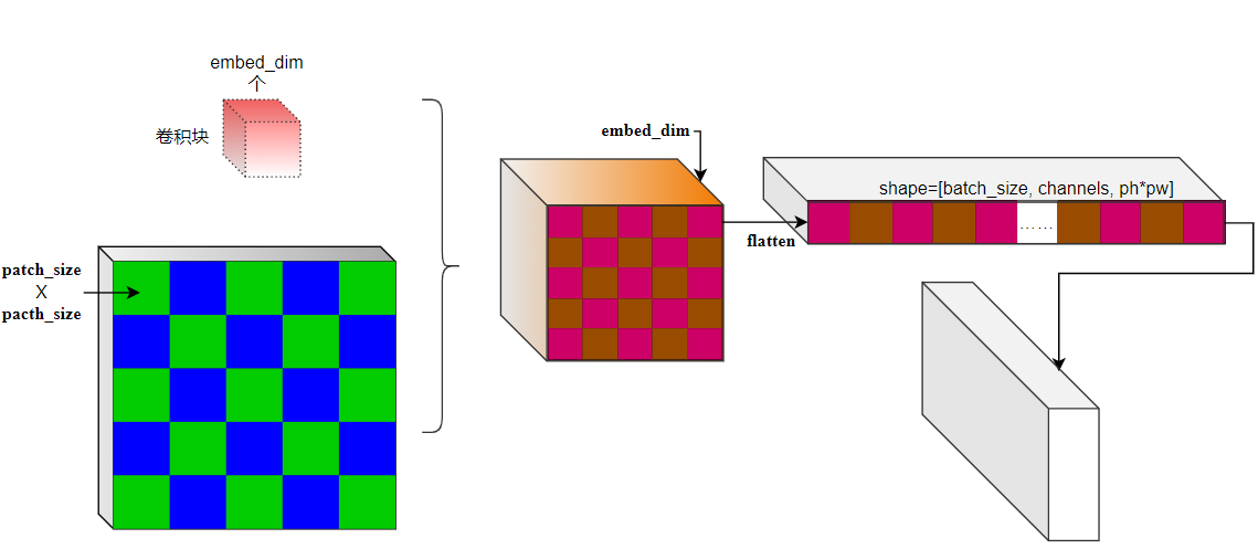
Summary PatchEmbed:
Pixel block coding mainly uses convolution to convolute on the original features, and then an optional BN layer. The size of convolution kernel of convolution is the size of pixel block, that is, patch_size, and the step size is also patch_size. In this way, there will be no information fusion between different pixel blocks, that is, only pixel blocks are encoded, which reduces a lot of convolution operations compared with the traditional CNN sliding window! The features after convolution are shown in the figure. Tile the tensor in the dimensions of dim=2 and dim=3, and transpose the last two dimensions to obtain the patch convolution output. Its shape is: (batch_size, ph*pw, channels). The BN layer is the BN layer in pytorch.
5.2 introduction to basiclayer
BasicLayer is well understood from the image. It is the generation unit of stage1~stage4 in the paper.
build layers:
self.layers = nn.ModuleList()
for i_layer in range(self.num_layers):
    layer = BasicLayer(dim=int(embed_dim * 2 ** i_layer),
                       input_resolution=(patches_resolution[0] // (2 ** i_layer),
                                         patches_resolution[1] // (2 ** i_layer)),
                       depth=depths[i_layer],
                       num_heads=num_heads[i_layer],
                       window_size=window_size,
                       mlp_ratio=self.mlp_ratio,
                       qkv_bias=qkv_bias, qk_scale=qk_scale,
                       drop=drop_rate, attn_drop=attn_drop_rate,
                       drop_path=dpr[sum(depths[:i_layer]):sum(depths[:i_layer + 1])],
                       norm_layer=norm_layer,
                       downsample=PatchMerging if (i_layer < self.num_layers - 1) else None,
                       use_checkpoint=use_checkpoint)
    self.layers.append(layer)
BasicLayer parameters:
"""
dim (int): Number of channels entered.
input_resolution (tuple[int]): Enter the resolution of the feature map.
depth (int): blocks Quantity, i.e. current stage Depth of.
num_heads (int): attention Number of headers.
window_size (int): shifted Size of local window.
mlp_ratio (float): mlp Dimension of hidden layer to embedding dim Ratio of.
qkv_bias (bool, optional): to query, key, value Add a learnable offset. default: True
qk_scale (float | None, optional): Override default qk scale of head_dim ** -0.5 if set.
drop (float, optional): Dropout rate. default: 0.0
attn_drop (float, optional): Attention dropout rate. default: 0.0
drop_path (float | tuple[float], optional): Stochastic depth rate. default: 0.0
norm_layer (nn.Module, optional): Normalization layer. default: nn.LayerNorm
downsample (nn.Module | None, optional): stay stage Finally, down sampling is performed Downsample layer. default: None
use_checkpoint (bool): Whether to use checkpoint Save the current layer. default: False.
"""
Each stage is composed of depth swintransformerblocks, just like the residual blocks in the residual neural network. In forward propagation, the basic layer is very simple. It uses SwinTransformerBlock to build the basic framework and an optional down sampling layer.
The introduction of SwinTransformerBlock is:
# build blocks
self.blocks = nn.ModuleList([
    SwinTransformerBlock(dim=dim, input_resolution=input_resolution,
                         num_heads=num_heads, window_size=window_size,
                         shift_size=0 if (i % 2 == 0) else window_size // 2,
                         mlp_ratio=mlp_ratio,
                         qkv_bias=qkv_bias, qk_scale=qk_scale,
                         drop=drop, attn_drop=attn_drop,
                         drop_path=drop_path[i] if isinstance(drop_path, list) else drop_path,
                         norm_layer=norm_layer)
    for i in range(depth)])
Here's self Blocks mainly contains the main SwinTransformerBlock blocks of the current stage.
The lower sampling layer is mainly used for pixel fusion.
# patch merging layer
if downsample is not None:
    self.downsample = downsample(input_resolution, dim=dim, norm_layer=norm_layer)
else:
    self.downsample = None
SwinTransformerBlock reference 5.3.
5.3 SwinTransformerBlock
Parameters:
"""
dim (int): Number of channels entered.
input_resolution (tuple[int]): Enter the resolution of the feature map.
num_heads (int): attention Number of headers.
window_size (int): Size of local window.
shift_size (int): SW-MSA Movement of size.
mlp_ratio (float): mlp Dimension of hidden layer to embedding dim Ratio of.
qkv_bias (bool, optional): to query, key, value Add a learnable offset. default: True
qk_scale (float | None, optional): Override default qk scale of head_dim ** -0.5 if set.
drop (float, optional): Dropout rate. default: 0.0
attn_drop (float, optional): Attention dropout rate. default: 0.0
drop_path (float, optional): Stochastic depth rate. default: 0.0
act_layer (nn.Module, optional): Active layer. default: nn.GELU
norm_layer (nn.Module, optional): Normalization layer.  default: nn.LayerNorm
"""
attn_mask
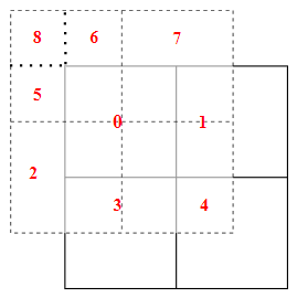
When shift_ When size is 0, attn_mask is None. When it is not 0, the original feature map will be divided into 9 regions due to the movement of the window. The division principle of these nine areas is: whether the source of the new window is generated by merging after moving. As input_resolution=(8,8) as an example, there are the following regional divisions:
# Generating all zero tensor
img_mask = torch.zeros((1, H, W, 1))
# mask by Region
h_slices = (slice(0, -self.window_size),
slice(-self.window_size, -self.shift_size),
slice(-self.shift_size, None))
w_slices = (slice(0, -self.window_size),
slice(-self.window_size, -self.shift_size),
slice(-self.shift_size, None))
cnt = 0
for h in h_slices:
for w in w_slices:
img_mask[:, h, w, :] = cnt
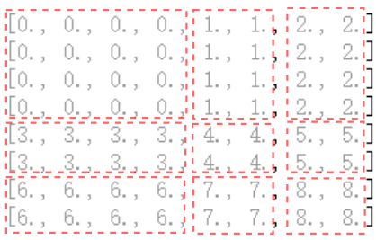
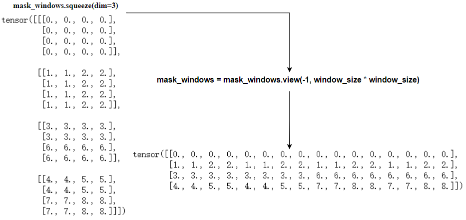
cnt += 1IMG at this time_ mask. Squeeze (dim = 3) is:
tensor([[[0., 0., 0., 0., 1., 1., 2., 2.],
         [0., 0., 0., 0., 1., 1., 2., 2.],
         [0., 0., 0., 0., 1., 1., 2., 2.],
         [0., 0., 0., 0., 1., 1., 2., 2.],
         [3., 3., 3., 3., 4., 4., 5., 5.],
         [3., 3., 3., 3., 4., 4., 5., 5.],
         [6., 6., 6., 6., 7., 7., 8., 8.],
         [6., 6., 6., 6., 7., 7., 8., 8.]]])
Then we can get the newly generated windows mask:
mask_windows = window_partition(img_mask, self.window_size)  # nW, window_size, window_size, 1
mask_windows = mask_windows.view(-1, self.window_size * self.window_size)
The mask of each newly generated window is:
attn_mask = mask_windows.unsqueeze(1) - mask_windows.unsqueeze(2)
attn_mask = attn_mask.masked_fill(attn_mask != 0, float(-100.0)).masked_fill(attn_mask == 0, float(0.0))
Attn here_ The mask will be passed to WindowAttention for multi head attention calculation in the window. In fact, the offset QKT/d − − √ + BQKT/d+B and a mask information will be added before softmax in WindowAttention. As shown in the last basis, set the mask value to − 100 − 100 for those points that are not equal to 0. In this way, a bias is generated for the window attention output generated by mobile splicing.
Forward propagation:
-
Step 1: check whether the defined input resolution is the same as l (sequence length) of the input characteristic image x;
-
Step 2: use self Norm1 normalizes the features, and then view the data (B, h, W, c);
-
Step 3: use torch Roll movement characteristic diagram;
-
Step 4: use window_partition partition window, which is in shifted_x is divided above to obtain the characteristic diagram of (num_windows*B, window_size, window_size, C), and then view(-1, self.window_size * self.window_size, C).
-
Step 5: realize W-MSA/SW-MSA} structure
# num_windows*B, window_size*window_size, C
attn_windows = self.attn(x_windows, mask=self.attn_mask)
Where x_windows is shifted_ Window division of X, self Attn is an instance of WindowAttention. The implementation difference of W-MSA/SW-MSA is whether to use shifted.
SwinTransformerBlock is mainly the implementation of W-MSA/SW-MSA. Its structure is LN+(W − MSA/SW − MSA)+LN+MLPLN+(W − MSA/SW − MSA)+LN+MLP. Note that the shifted feature map will be restored at last. LN here is NN LayerNorm; MLP is the author's own implementation.
MLP:
MLP is: full connection layer + activation layer + Dropout layer + full connection layer + Dropout layer
self.fc1 = nn.Linear(in_features, hidden_features)
self.act = act_layer()
self.fc2 = nn.Linear(hidden_features, out_features)
self.drop = nn.Dropout(drop)
5.4 WindowAttention
Moving / non moving window attention model based on multi head attention model with relative position offset.
Parameters:
"""
dim (int): Number of input channels.
window_size (tuple[int]): Size of local window.
num_heads (int): attention Number of headers.
qkv_bias (bool, optional):  to query, key, value Add a learnable offset. default: True
qk_scale (float | None, optional): Override default qk scale of head_dim ** -0.5 if set
attn_drop (float, optional): Dropout ratio of attention weight. default: 0.0
proj_drop (float, optional): Dropout ratio of output. default: 0.0
"""
Initialization of window attention layer:
Relative position offset
# 2*Wh-1 * 2*Ww-1, nH
self.relative_position_bias_table = nn.Parameter(
   torch.zeros((2 * window_size[0] - 1) * (2 * window_size[1] - 1), num_heads))
trunc_normal_(self.relative_position_bias_table, std=.02)
self.relative_position_bias_table is initialized with truncated positive distribution, and the standard deviation is 0.02.
As shown in the paper, if MM identifies the size of the window, the initialized offset matrix is B ^∈ R (2m − 1) × (2M−1)B^∈R(2M−1) × (2m − 1), why (2m − 1) × (2M−1)(2M−1) × (2M−1)? This problem will be explained later!
The most important thing of WindowAttention layer is that the coding part of relative position offset is relatively complex. Other operations are familiar with torch layer. Therefore, here we study its processing process carefully.
The relative position offset BB is a token from B^B ^. Therefore, B^B ^ stores all offsets, and BB should be obtained through index. The following is the index generation:
coords: records the coordinates of the window, and the origin is the upper left corner of the window;
coords_flatten: records the tiling of coordinates; sahpe is (2, M2);
relative_coords: records the relative position of pixels (pixel blocks) in the window; For example, there are M2 relative positions in the pixel block , patchapatcha , because there are M2 pixel blocks in the window.
The author's implementation method in the project is:
relative_coords = coords_flatten[:, :, None] - coords_flatten[:, None, :]
relative_coords = relative_coords.permute(1, 2, 0).contiguous()
Therefore, relative_ The shape of coords is (M2M2, M2M2, 2). Relative at this time_ Coords [0,:,:] identifies the relative coordinates from (h, w)=(0, 0) to all points. Note that we have the relative positions of any two coordinates in the window!
However, the author has carried out the following operations:
relative_coords[:, :, 0] += self.window_size[0] - 1
relative_coords[:, :, 1] += self.window_size[1] - 1
relative_coords[:, :, 0] *= 2 * self.window_size[1] - 1
What the first two lines do is move the relative left to start from 0. The third line multiplies the relative coordinates of height H by 2M − 12M − 1.
What is the meaning of multiplying 2M − 12M − 1? self.relative_position_bias_table is an initialized offset table. We need to use an index to get it, and relative_coords is the key to index generation. The code for index generation is:
relative_position_index = relative_coords.sum(-1)
The index here is essentially the same as the offset. If the indexes are the same, the offset is the same. First, we discuss relative_ position_ What kind of nature should index have
-
When the pixel block patcha is in the same row (or in the same column) as the pixel block patcha+1; When the pixel block patchb is in the same row (or in the same column) as the pixel block patchb+1. The offset between pixel block {patcha and pixel block} patchb should be the same as that between pixel block} patcha+1 and pixel block} patchb+1! Namely:
relative_position_index[i,j] = relative_position_index[M-1-j,M-1-i]
Note that the above equation should satisfy most cases, but not on the boundary of W, because our data is row first, and the index + 1 is the next pixel block. If the current boundary is wide, the next pixel block will wrap. Therefore, our index should preferably satisfy that the remainder of j+1j+1 divided by ll is not 0, where l ∈ {M,2M,..., M2}.
The more cumbersome thing is that the next line breaks on the wide right boundary, but in this mode, the offset should be the same! For example, the offset of 3M − 1 pixel block relative to the 0th pixel block and the offset of 4M − 1 pixel block relative to the mmth pixel block are the same!
-
So the question is, based on the above criteria, how many offsets do we need at least? We know from the paper that (2M − 1) is required × (2M − 1) PCs. How is this calculated?
First, relative_ position_ The shape of the index matrix is (M2M2, M2M2). In the main diagonal direction, we have 2M2 − 12M2 − 1 line, and each line has only one or two offset indexes. Refer to the above rule description for the reason. So what are 1 and 2? It can be found from the derivation that the sequence of offset index number of each line is:
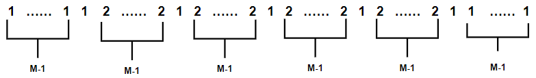
The number of this sequence 2 is 2(M − 1) × (M−1); The quantity of 1 is: 2(M − 1)+2M − 1.
Therefore, the number of indexes we need is:
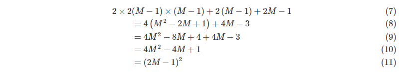
In fact, we probably know that multiplying 2M − 12M − 1 is to make the index meet the above requirements, and the minimum value to maximum value of the index is continuous! When it is less than 2M − 12M − 1, the index matrix cannot meet the above rules; When it is greater than 2M − 12M − 1, the value of the index matrix is not continuous! So why 2M − 12?
Explanation:
-
(1) On the characteristic graph corresponding to high H, each m × The blocks of M are the same, and the main diagonal direction is the same, so 2M − 1 different m will be generated × The index block of the ordinate H of M;
-
(2) Appeal high every M × The wide index blocks corresponding to M blocks are the same;
-
(3) An M × M wide index block, and its wide index value range is [0,2M − 2];
-
(4) For indexes, we use: H × If the final relative position index is obtained in the form of x+W, then we multiply x for each row, and we still need to keep its adjacent M × For the size relationship between M blocks, for high h, the difference between adjacent high indexes is 1. Assuming that the row index of the current block is m, there are:
mx+0>(m−1)x+2M−2⇒x>2M−2 -
(5) For relative_ The lower left element of coords, after combining the high index and wide index, is:
(2M−2)x+2M−2≤(2M−1)2⇒x≤2M−1 -
(6) From inequalities (6) and (7), it can be concluded that the number of multipliers can only be 2M − 1.
-
So far, we have obtained the index of relative position offset, such as M=4. We can get the following index:
tensor([[24, 23, 22, 21, 17, 16, 15, 14, 10,  9,  8,  7,  3,  2,  1,  0],
        [25, 24, 23, 22, 18, 17, 16, 15, 11, 10,  9,  8,  4,  3,  2,  1],
        [26, 25, 24, 23, 19, 18, 17, 16, 12, 11, 10,  9,  5,  4,  3,  2],
        [27, 26, 25, 24, 20, 19, 18, 17, 13, 12, 11, 10,  6,  5,  4,  3],
        [31, 30, 29, 28, 24, 23, 22, 21, 17, 16, 15, 14, 10,  9,  8,  7],
        [32, 31, 30, 29, 25, 24, 23, 22, 18, 17, 16, 15, 11, 10,  9,  8],
        [33, 32, 31, 30, 26, 25, 24, 23, 19, 18, 17, 16, 12, 11, 10,  9],
        [34, 33, 32, 31, 27, 26, 25, 24, 20, 19, 18, 17, 13, 12, 11, 10],
        [38, 37, 36, 35, 31, 30, 29, 28, 24, 23, 22, 21, 17, 16, 15, 14],
        [39, 38, 37, 36, 32, 31, 30, 29, 25, 24, 23, 22, 18, 17, 16, 15],
        [40, 39, 38, 37, 33, 32, 31, 30, 26, 25, 24, 23, 19, 18, 17, 16],
        [41, 40, 39, 38, 34, 33, 32, 31, 27, 26, 25, 24, 20, 19, 18, 17],
        [45, 44, 43, 42, 38, 37, 36, 35, 31, 30, 29, 28, 24, 23, 22, 21],
        [46, 45, 44, 43, 39, 38, 37, 36, 32, 31, 30, 29, 25, 24, 23, 22],
        [47, 46, 45, 44, 40, 39, 38, 37, 33, 32, 31, 30, 26, 25, 24, 23],
        [48, 47, 46, 45, 41, 40, 39, 38, 34, 33, 32, 31, 27, 26, 25, 24]])
Other initialization
self.qkv = nn.Linear(dim, dim * 3, bias=qkv_bias)
self.attn_drop = nn.Dropout(attn_drop)
self.proj = nn.Linear(dim, dim)
self.proj_drop = nn.Dropout(proj_drop)
Forward propagation:
-
First get q, k, v.
self.qkv = nn.Linear(dim, dim * 3, bias=qkv_bias)
Note that linear transformation is used here to expand the dimension to 3 times and make it correspond to Q, K and V.
Code block generating q, k, v:
qkv = self.qkv(x).reshape(B_, N, 3, self.num_heads, C // self.num_heads).permute(2, 0, 3, 1, 4)
q, k, v = qkv[0], qkv[1], qkv[2]
Note that the shape of x here is (num_windows*B, N, C), and the above 3 can be understood as dividing the newly generated channels into Q, K and V, and then dividing the number of channels C of each into: self num_ Heads and C / / self num_ Heads two dimensions to implement the multi head mechanism.
-
Calculation attention: QK^T / √ d
q = q * self.scale
attn = (q @ k.transpose(-2, -1))
-
Add bias to attention
relative_position_bias = self.relative_position_bias_table[ self.relative_position_index.view(-1)].view( self.window_size[0] * self.window_size[1], self.window_size[0] * self.window_size[1], -1) # Wh*Ww,Wh*Ww,nH relative_position_bias = relative_position_bias.permute(2, 0, 1).contiguous() # nH, Wh*Ww, Wh*Ww attn = attn + relative_position_bias.unsqueeze(0) -
Achieve multi head attention
Attention(Q,K,V)=SoftMax(QKT/d−−√+B)VAttention(Q,K,V)=SoftMax(QKT/d+B)V
Over!