
Data link: https://pan.baidu.com/s/1gE4JvsgK5XV-G9dGpylcew
Extraction code: y409
Project background
1. Titanic: an Olympic class cruise ship under the jurisdiction of British white star shipping company. It was built at Harland and Wolff shipyard in Belfast port, Ireland on March 31, 1909. It was launched on May 31, 1911 and completed the trial voyage on April 2, 1912.
2. Maiden voyage time: April 10, 1912
3. Route: starting from Southampton, UK, via Cherbourg Oakville, France and Queenstown, Ireland, to New York, USA.
4. Shipwreck: April 15, 1912 (hit the iceberg at about 23:40 on April 14, 1912)
Crew + passengers: 2224
5. Number of victims: 1502 (67.5%)
target
According to the characteristics of each passenger in the training set and the corresponding relationship between the rescue signs, the training model predicts whether the passengers in the test set are rescued. (binary classification problem)
data dictionary
1, Base field
PassengerId passenger id:
Training set 891 (1 - 891), test set 418 (892 - 1309)
Whether the Survived was rescued:
1 = yes, 0 = no
Rescued: 38%
Death rate: 62% (actual death rate: 67.5%)
Pclass ticket level:
Represents socio-economic status. 1 = advanced, 2 = intermediate, 3 = low
1 : 2 : 3 = 0.24 : 0.21 : 0.55
Name Name:
Example: Futrelle, Mrs. Jacques Heath (Lily May Peel)
Example: Heikkinen, miss Laina
Sex:
male 577, female 314
Male: female = 0.65: 0.35
Age (20% missing):
Training set: 714 / 891 = 80%
Test set: 332 / 418 = 79%
Total siblings or spouses of SibSp peers:
68% none, 23% have 1... Up to 8
Total number of parents or children of Parch peers:
76% none, 13% 1, 9% 2... Up to 6
Some children travelled only with a nanny, therefore parch=0 for them.
Ticket number (inconsistent format):
Example: A/5 21171
Example: ton / O2 three million one hundred and one thousand two hundred and eighty-two
Fare at far:
The test set is missing a data
Cabin No.:
There are only 204 data in the training set and 91 data in the test set
Example: C85
Embarked boarding port:
C = Cherbourg 19%, Q = Queenstown 9%, S = Southampton 72%
The training set is less than two data
2, Derived fields (part, supplemented in subsequent codes)
Title Title:
dataset.Name.str.extract( " ([A-Za-z]+).", expand = False)
Extracted from names, related to names and social status
FamilySize family size:
Parch + SibSp + 1
The intermediate feature of IsAlone feature used to calculate whether to travel alone is reserved for the time being
IsAlone alone:
FamilySize == 1
Do you travel alone
HasCabin has independent Cabin:
It is uncertain whether the sample without CabinId has no cabin or the data is true
Characteristic Engineering
Classifying:
Sample classification or grading
Correlating:
The correlation degree between sample prediction results and features, and the correlation degree between features
Converting:
Feature transformation (vectorization)
Completing:
Complete estimation of missing characteristic values
Correcting:
The abnormal data with obvious outliers or obvious inclination of prediction results shall be corrected or excluded
Creating:
New features are derived from existing features to meet the requirements of relevance, vectorization and integrity
Charting:
Select the correct visual chart according to the nature of data and problem objectives
feature analysis
1, Import necessary Libraries
# Import library
# Data analysis and exploration
import pandas as pd
import numpy as np
import random as rnd

# visualization
import seaborn as sns
import matplotlib.pyplot as plt
%matplotlib inline

# Eliminate warning
import warnings
warnings.filterwarnings('ignore')

# Machine learning model
# Logistic regression model
from sklearn.linear_model import LogisticRegression
# Linear classification support vector machine
from sklearn.svm import SVC, LinearSVC
# Random forest classification model
from sklearn.ensemble import RandomForestClassifier
# K-nearest neighbor classification model
from sklearn.neighbors import KNeighborsClassifier
# Bayesian classification model
from sklearn.naive_bayes import GaussianNB
# Perceptron model
from sklearn.linear_model import Perceptron
# Gradient descent algorithm
from sklearn.linear_model import SGDClassifier
# Decision tree model
from sklearn.tree import DecisionTreeClassifier
2, Import data
# Get data, training set, train_df, test set_ df
train_df = pd.read_csv('E:/PythonData/titanic/train.csv')
test_df = pd.read_csv('E:/PythonData/titanic/test.csv')
combine = [train_df, test_df]
train_df and test_df is merged into combine (for unified processing of features: for df in combine:)
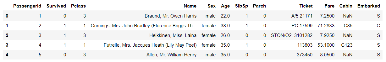
3, View data
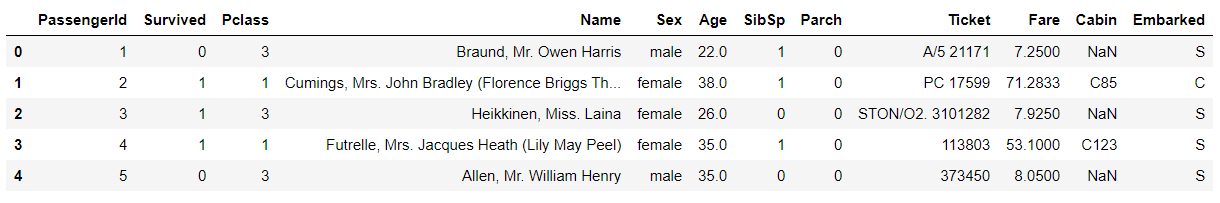
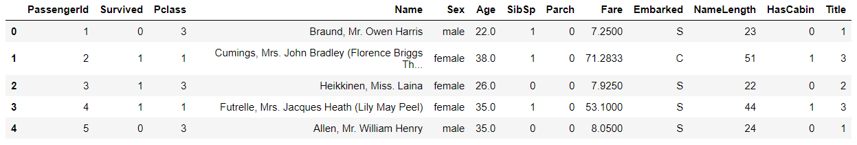
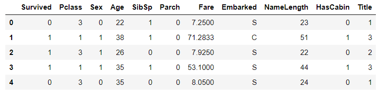
# Explore data
# View field structure, type and head examples
train_df.head()
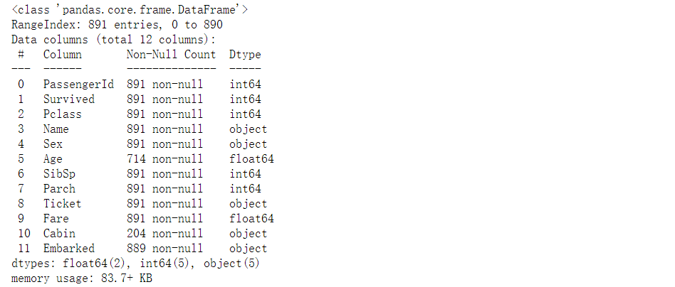
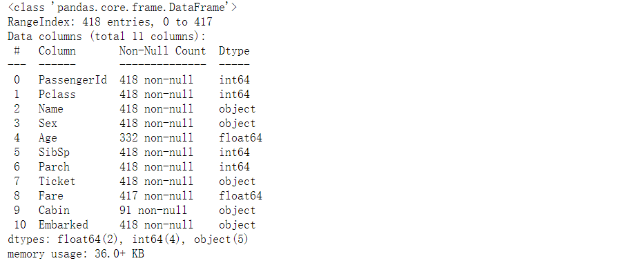
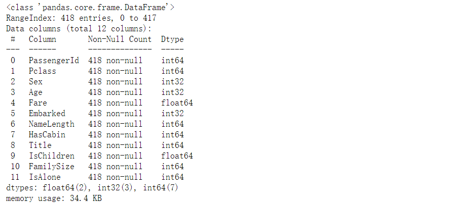
4, View field information
# View the non empty sample size and field type of each feature
train_df.info()
print("*"*40)
test_df.info()
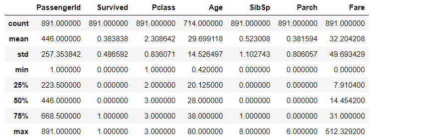
5, View field statistics
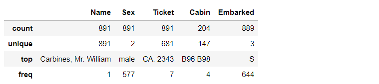
# View the data distribution of numeric class (int, float) features
train_df.describe()
# View the data distribution of non numeric class (object type) features
train_df.describe(include=["O"])
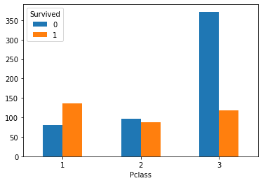
6, Check the relationship between cabin level and survival
1. Create a cabin class and survival contingency table
#Generate pclass_ Contingency table of survived
Pclass_Survived = pd.crosstab(train_df['Pclass'], train_df['Survived'])

2. Draw the bar chart of cabin class and survival
# Draw bar chart
Pclass_Survived.plot(kind = 'bar')
plt.xticks(rotation=360)
plt.show()
3. Check the bar chart of survival rate of different cabin classes
train_df[["Pclass","Survived"]].groupby(["Pclass"],as_index=True).mean().sort_values(by="Pclass",ascending=True).plot()
plt.xticks(range(1,4)[::1])
plt.show()
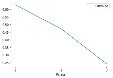
Analysis: 1, 2 and 3 represent the class 1, class 2 and class 3 respectively. The rich and middle class have a higher survival rate, while the survival rate at the bottom is low.
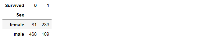
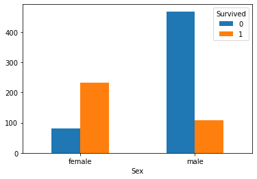
7, Look at the relationship between gender and survival
1. Create a contingency table of gender and survival
#Generate gender and survival contingency table
Sex_Survived = pd.crosstab(train_df['Sex'],train_df['Survived'])
2. Draw a bar graph of gender and survival
Sex_Survived.plot(kind='bar')

# Abscissa 0 and 1 represent male and female respectively
plt.xticks(rotation=360)
plt.show()
3. The table of gender and survival rate is as follows:
# View gender and survival
train_df[["Sex","Survived"]].groupby(["Sex"],as_index=False).mean().sort_values(by="Survived",ascending=False)
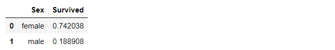
Analysis: gender is strongly related to survival. The survival rate of female users is significantly higher than that of men.
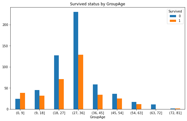
8, Check the relationship between passenger age and survival
1. Missing age of the year (median instead of missing data)
# The median age was used to replace the missing age value
Agemedian = train_df['Age'].median()

#Populates the current table with missing values
train_df.Age.fillna(Agemedian, inplace = True)

#Reset index
train_df.reset_index(inplace = True)
2. Group ages and draw a bar graph of age and number of survivors
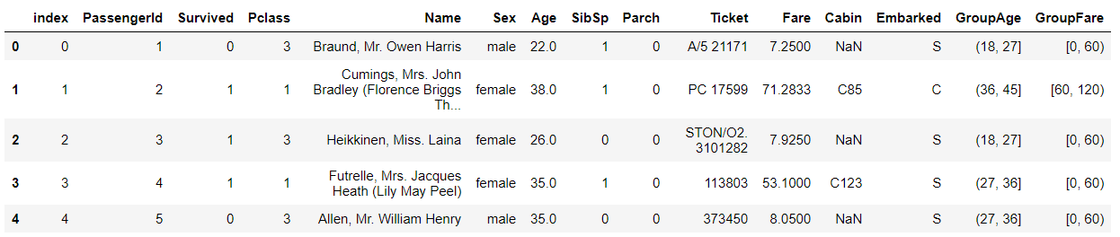
#Group Age: 2 * * 10 > 891 is divided into 10 groups, and the group distance is (maximum 80 - Minimum 0) / 10 = 8, taking 9
bins = [0, 9, 18, 27, 36, 45, 54, 63, 72, 81, 90]

train_df['GroupAge'] = pd.cut(train_df.Age, bins)

GroupAge_Survived = pd.crosstab(train_df['GroupAge'], train_df['Survived'])
GroupAge_Survived.plot(kind = 'bar',figsize=(10,6))

plt.xticks(rotation=360)
plt.title('Survived status by GroupAge')
3. Draw the line chart of survival rate corresponding to different ages
# Number of survivors of different ages
GroupAge_Survived_1 = GroupAge_Survived[1]
# Survival rate of different age groups
GroupAge_all = GroupAge_Survived.sum(axis=1)
GroupAge_Survived_rate = round(GroupAge_Survived_1/GroupAge_all,2)
GroupAge_Survived_rate.plot(figsize=(10,6))
plt.show()
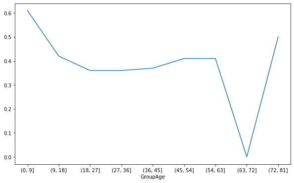
Analysis: the survival rate was higher in the age group of 0-9 and 72-81 years. Explain that the elderly and children are preferred when escaping. However, the survival rate corresponding to 63-72 is the lowest, which is caused by too few people in the corresponding age group.
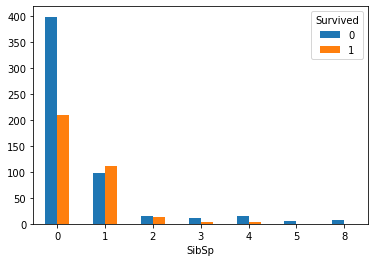
9, Check the relationship between the number of siblings and spouses and survival
1. Create a contingency table for the number of siblings and spouses and survival
# Generate contingency table
SibSp_Survived = pd.crosstab(train_df['SibSp'], train_df['Survived'])
SibSp_Survived

2. Draw a bar chart of the number of siblings and spouses and survival
SibSp_Survived.plot(kind='bar')

plt.xticks(rotation=360)
plt.show()
3. Draw a broken line chart between the number of siblings and spouses and survival rate
# Look at the relationship between the number of sibling spouses and survival rate
train_df[["SibSp","Survived"]].groupby(["SibSp"],as_index=True).mean().sort_values(by="SibSp",ascending=True).plot()
plt.show()
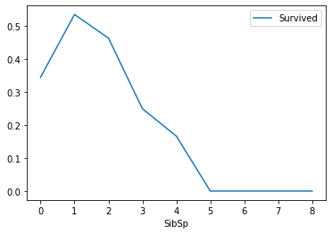
Analysis: the survival rate corresponding to the number of siblings and spouses from 1-2 is higher, and the others are relatively lower.
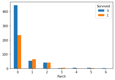
10, Look at the relationship between the number of parents and children and survival
1. Create a contingency table for the number and survival of parents and children
Create contingency table
Parch_Survived = pd.crosstab(train_df['Parch'], train_df['Survived'])
Parch_Survived

2. Draw a histogram of the number and survival of parents and children
Parch_Survived.plot(kind='bar')

plt.xticks(rotation=360)
plt.show()
3. Draw a broken line chart of the number of parents and children and survival rate
# Look at the relationship between the number of parents and children and survival
train_df[["Parch","Survived"]].groupby(["Parch"],as_index = True).mean().sort_values(by="Parch",ascending=True).plot()
plt.show()
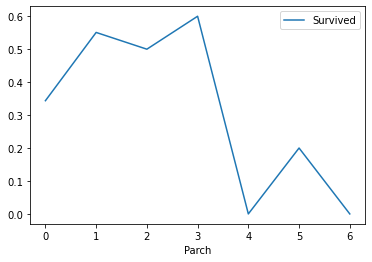
Analysis: when the number of parents and children is 1-3, the corresponding survival rate is higher, and others are relatively lower
11, Check the relationship between different ticket prices and survival
1. Divide the ticket price and create the survival contingency table corresponding to different tickets
#Group Fare: 2 * * 10 > 891 is divided into 10 groups. The group distance is (maximum 512.3292 - Minimum 0) / 10, and the value is 60
bins = [0, 60, 120, 180, 240, 300, 360, 420, 480, 540, 600]
train_df['GroupFare'] = pd.cut(train_df.Fare, bins, right = False)
GroupFare_Survived = pd.crosstab(train_df['GroupFare'], train_df['Survived'])
GroupFare_Survived
2. Draw cluster column chart of survival quantity corresponding to different ticket prices
# Draw a clustered column
GroupFare_Survived.plot(kind = 'bar',figsize=(10,6))

# Adjust scale
plt.xticks(rotation=360)
plt.title('Survived status by GroupFare')

GroupFare_Survived.iloc[2:].plot(kind = 'bar',figsize=(10,6))
# Adjust scale
plt.xticks(rotation=360)
plt.title('Survived status by GroupFare(Fare>=120)')
3. Draw a broken line chart of survival rate corresponding to non fare
# Draw a broken line chart of survival rate corresponding to ticket price

# Survival number corresponding to different fares
GroupFare_Survived_1 = GroupFare_Survived[1]
# Survival rate corresponding to different fares
GroupFare_all = GroupFare_Survived.sum(axis=1)
GroupFare_Survived_rate = round(GroupFare_Survived_1/GroupFare_all,2)
GroupFare_Survived_rate.plot()
plt.show()
Analysis: the survival rate is higher when the ticket price is 120-180 and 480-540, and there is a positive correlation between the ticket price and the survival rate.
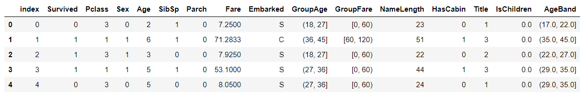
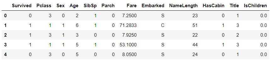
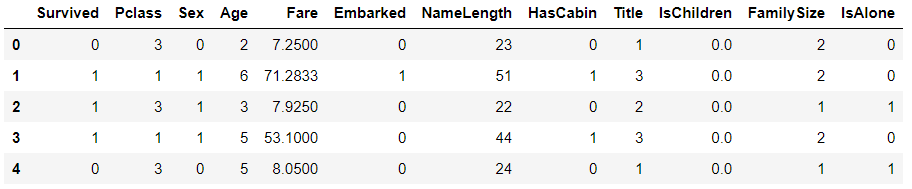
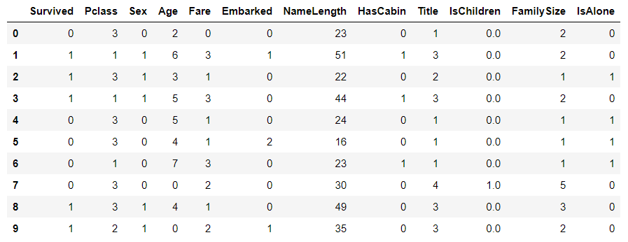
train_df.head()
Remove the fields such as index, GroupAge, GroupFare, etc
train_df = train_df.drop(["index","GroupAge","GroupFare"],axis=1)
train_df.head()
Characteristic cleaning
1.NameLength
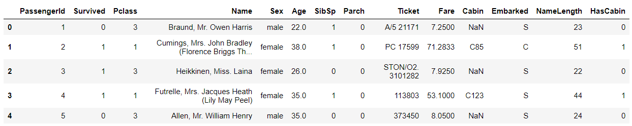
# Create training set and test set name length fields
train_df['NameLength'] = train_df['Name'].apply(len)
test_df['NameLength'] = test_df['Name'].apply(len)
Note: it is explained here that the Kaggle author uses the name field as one of the features because the name contains the passenger's title. The longer the name, the more titles corresponding to it. That is, the corresponding social status is high.
2.HasCabin (whether there is a cabin)
Classify whether passengers have cabins into two categories
# Using anonymous functions, NaN is a floating-point type, 0 if it is a floating-point type, otherwise 1 (i.e. 0 if there is no cabin, 1 if there is a cabin)
train_df['HasCabin'] = train_df["Cabin"].apply(lambda x: 0 if type(x) == float else 1)
test_df['HasCabin'] = test_df["Cabin"].apply(lambda x: 0 if type(x) == float else 1)
train_df.head()
Delete Ticket and Cabin
The Ticket and Cabin fields are deleted because the Ticket field represents the name of the Ticket. There was no correlation with passenger survival. Bin is deleted because the bin field is replaced by hasbin.
# Eliminate the two features of Ticket (no correlation by human judgment) and Cabin (too little effective data)
train_df = train_df.drop(["Ticket","Cabin"],axis=1)
test_df = test_df.drop(["Ticket","Cabin"],axis=1)
combine = [train_df,test_df]
print(train_df.shape,test_df.shape,combine[0].shape,combine[1].shape)

3.Title Field
# Create a Title Feature Based on the name, which will contain gender and class information
# dataset. Name. str.extract(' ([A-Za-z]+)\.' ->  Start with a space Extract the ending string
# Match with gender, and see whether various titles belong to men or women respectively, which is convenient for subsequent classification

for dataset in combine:
    dataset['Title'] = dataset.Name.str.extract(' ([A-Za-z]+)\.', expand=False)
pd.crosstab(train_df['Title'], train_df['Sex']).sort_values(by=["male","female"],ascending=False)

Classify passengers with different titles
# Classify the titles as Mr, miss, Mrs, master, rare_ Male,Rare_ Female (rare is distinguished by male and female)
for dataset in combine:
    dataset["Title"] = dataset["Title"].replace(['Lady', 'Countess', 'Dona'],"Rare_Female")
    dataset["Title"] = dataset["Title"].replace(['Capt', 'Col','Don','Dr','Major',
                                                 'Rev','Sir','Jonkheer',],"Rare_Male")
    dataset["Title"] = dataset["Title"].replace('Mlle', 'Miss')
    dataset['Title'] = dataset['Title'].replace('Ms', 'Miss')
    dataset['Title'] = dataset['Title'].replace('Mme', 'Miss')
Draw the survival rate corresponding to different titles
# Summarize and calculate the mean value of Survived by Title to view the correlation
T_S = train_df[["Title","Survived"]].groupby(["Title"],as_index=False).mean().sort_values(by='Survived',ascending=True)
plt.figure(figsize=(10,6))
plt.bar(T_S['Title'],T_S['Survived'])
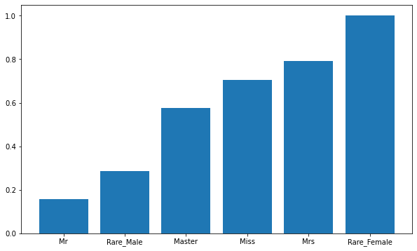
Analysis: the titles are Miss, Mrs and Rare_Female passengers have a high survival rate, which means that when escaping, we follow the principle of giving priority to women.
Map Title features to numeric values
title_mapping = {"Mr":1,"Miss":2,"Mrs":3,"Master":4,"Rare_Female":5,"Rare_Male":6}
for dataset in combine:
    dataset["Title"] = dataset["Title"].map(title_mapping)
    dataset["Title"] = dataset["Title"].fillna(0)
    # To avoid routine operations with empty data
train_df.head()
Delete name field
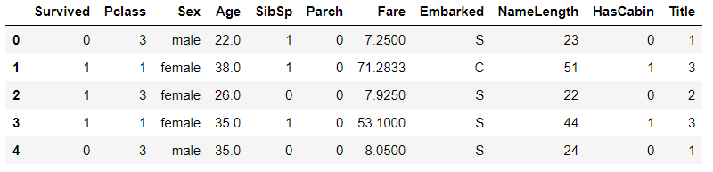
# The Name field can be eliminated
# The PassengerId field of the training set is only a self increasing field, which has nothing to do with prediction and can be eliminated
train_df = train_df.drop(["Name","PassengerId"],axis=1)
test_df = test_df.drop(["Name"],axis=1)
train_df.head()
# Re combine each time you delete a feature
combine = [train_df,test_df]
combine[0].shape,combine[1].shape

4.sex field
Convert the gender field to a numeric value, setting women to 0 and men to 1
# sex features are mapped to numeric values
for dataset in combine:
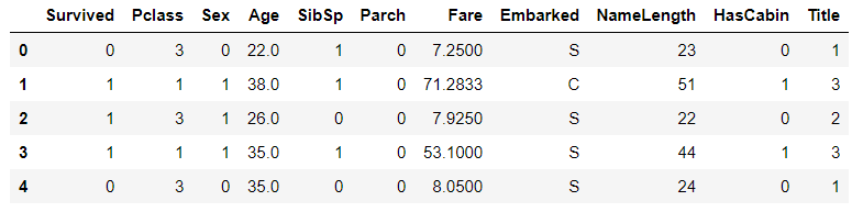
dataset["Sex"] = dataset["Sex"].map({"female":1,"male":0}).astype(int)
# Add astype(int) after to avoid Boolean processing?
train_df.head()
5.Age field
guess_ages = np.zeros((6,3))
guess_ages
Null the Age field (filled with the Age median of the same Pclass and Title)
# Fill in the null value of the age field
# Replace with the Age median of the same Pclass and Title (for combinations with empty median, replace with the overall median of Title)

for dataset in combine:
    # Take the median of 6 combinations
    for i in range(0, 6):

        for j in range(0, 3):
            guess_title_df = dataset[dataset["Title"]==i+1]["Age"].dropna()

            guess_df = dataset[(dataset['Title'] == i+1) & (dataset['Pclass'] == j+1)]['Age'].dropna()

            # age_mean = guess_df.mean()
            # age_std = guess_df.std()
            # age_guess = rnd.uniform(age_mean - age_std, age_mean + age_std)

            age_guess = guess_df.median() if ~np.isnan(guess_df.median()) else guess_title_df.median()
            #print(i,j,guess_df.median(),guess_title_df.median(),age_guess)
            # Convert random age float to nearest .5 age
            guess_ages[i,j] = int( age_guess/0.5 + 0.5 ) * 0.5
    # Assign a value to the Age field that meets the conditions in 6
    for i in range(0, 6):
        for j in range(0, 3):
            dataset.loc[ (dataset.Age.isnull()) & (dataset.Title == i+1) & (dataset.Pclass == j+1),
                        'Age'] = guess_ages[i,j]

    dataset['Age'] = dataset['Age'].astype(int)

train_df.head()
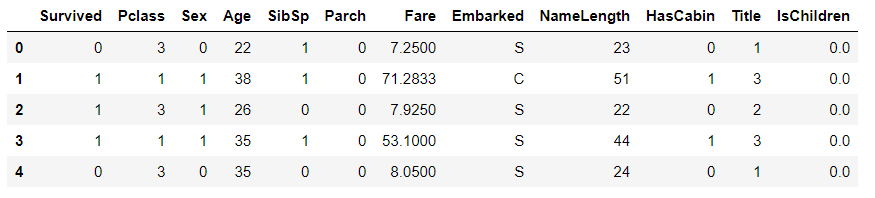
6. IsChildren (child or not)
Children younger than or equal to 12 are regarded as children, and the rest are non children. Represented by 1 and 0 respectively
#Create child feature
for dataset in combine:
    dataset.loc[dataset["Age"] > 12,"IsChildren"] = 0
    dataset.loc[dataset["Age"] <= 12,"IsChildren"] = 1
train_df.head()
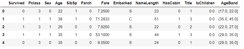
Age range
# Create age range characteristics
# pd.cut is evenly divided according to the size of the value. The size of each value interval is the same, but the number of samples may be different
# pd.qcut is divided according to the distribution frequency of samples on the value, and the number of samples in each group is the same
train_df["AgeBand"] = pd.qcut(train_df["Age"],8)
train_df.head()
train_df[["AgeBand","Survived"]].groupby(["AgeBand"],as_index = False).mean().sort_values(by="AgeBand",ascending=True)

Convert age range to numeric value
# Normalize the age range to 0 to 4
for dataset in combine:
    dataset.loc[ dataset['Age'] <= 17, 'Age'] = 0
    dataset.loc[(dataset['Age'] > 17) & (dataset['Age'] <= 21), 'Age'] = 1
    dataset.loc[(dataset['Age'] > 21) & (dataset['Age'] <= 25), 'Age'] = 2
    dataset.loc[(dataset['Age'] > 25) & (dataset['Age'] <= 26), 'Age'] = 3
    dataset.loc[(dataset['Age'] > 26) & (dataset['Age'] <= 31), 'Age'] = 4
    dataset.loc[(dataset['Age'] > 31) & (dataset['Age'] <= 36.5), 'Age'] = 5
    dataset.loc[(dataset['Age'] > 36.5) & (dataset['Age'] <= 45), 'Age'] = 6
    dataset.loc[ dataset['Age'] > 45, 'Age'] = 7
train_df.head()
Remove AgeBand field
# Remove AgeBand feature
train_df = train_df.drop('GroupAge',axis=1)
combine = [train_df,test_df]
train_df.head()
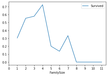
7.FamilySize (combine the total number of siblings or spouses and the total number of parents or children into one feature)
# Create a family size FamilySize combination feature + 1 is to consider yourself
for dataset in combine:
    dataset["FamilySize"] = dataset["Parch"] + dataset["SibSp"] + 1
train_df[["FamilySize","Survived"]].groupby(["FamilySize"],as_index = True).mean().sort_values(by="FamilySize",ascending=True).plot()
plt.xticks(range(12)[::1])
plt.show()
Draw a broken line graph of FamilySize and survival rate
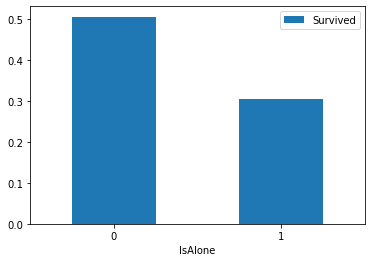
8.IsAlone (alone or not)
# Create IsAlone feature alone
for dataset in combine:
    dataset["IsAlone"] = 0
    dataset.loc[dataset["FamilySize"] == 1,"IsAlone"] = 1
train_df[["IsAlone","Survived"]].groupby(["IsAlone"],as_index=True).mean().sort_values(by="IsAlone",ascending=True).plot(kind='bar')
plt.xticks(rotation=360)
plt.show()
Check whether one person alone is associated with the survival histogram
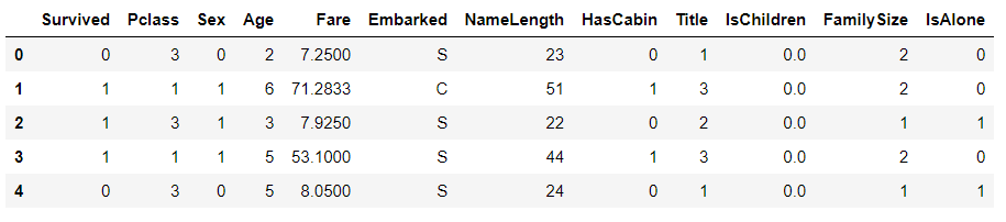
Remove Parch,Sibsp field
train_df = train_df.drop(["Parch","SibSp"],axis=1)
test_df = test_df.drop(["Parch","SibSp"],axis=1)
combine = [train_df,test_df]
train_df.head()
9.Embarked (Port factor)
# Add null value to Embarked
# Get the port with the most ships
freq_port = train_df["Embarked"].dropna().mode()[0]
freq_port

Process missing values (fill in missing values with modes)
for dataset in combine:
    dataset["Embarked"] = dataset["Embarked"].fillna(freq_port)
Create contingency table
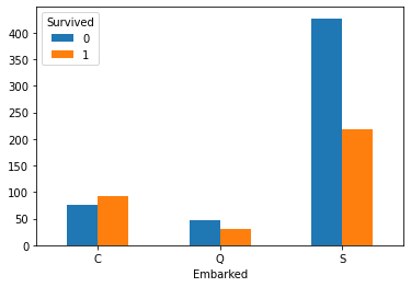
Embarked_Survived = pd.crosstab(train_df['Embarked'],train_df['Survived'])
Embarked_Survived

Draw the bar chart of survival corresponding to different ports
Embarked_Survived.plot(kind='bar')

plt.xticks(rotation=360)
plt.show()
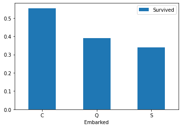
Draw bar charts of different ports and survivals
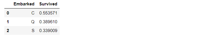
# View the relationship between different ports and survivals
train_df[["Embarked","Survived"]].groupby(["Embarked"],as_index=True).mean().sort_values(by="Embarked",ascending=True).plot(kind='bar')
plt.xticks(rotation=360)
plt.show()
Convert Embarked to numeric value
# Digitize Embarked
for dataset in combine:
    dataset["Embarked"] = dataset["Embarked"].map({"S":0,"C":1,"Q":2}).astype(int)
train_df.head()
9.Fare
# Fill in null values for Fare in the test set, using the median
test_df["Fare"].fillna(test_df["Fare"].dropna().median(),inplace=True)
test_df.info()
Set different fare ranges
# Create FareBand interval feature
train_df["FareBand"] = pd.qcut(train_df["Fare"],4)
train_df[["FareBand","Survived"]].groupby(["FareBand"],as_index=False).mean().sort_values(by="FareBand",ascending=True)

Digitize the sections where different fares are located
# Convert Fare features to ordinal values according to FareBand
for dataset in combine:
    dataset.loc[ dataset['Fare'] <= 7.91, 'Fare'] = 0
    dataset.loc[(dataset['Fare'] > 7.91) & (dataset['Fare'] <= 14.454), 'Fare'] = 1
    dataset.loc[(dataset['Fare'] > 14.454) & (dataset['Fare'] <= 31), 'Fare']   = 2
    dataset.loc[ dataset['Fare'] > 31, 'Fare'] = 3
    dataset['Fare'] = dataset['Fare'].astype(int)

# Remove FareBand
train_df = train_df.drop(['FareBand'], axis=1)
combine = [train_df, test_df]

train_df.head(10)
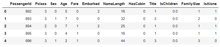
test_df.head()
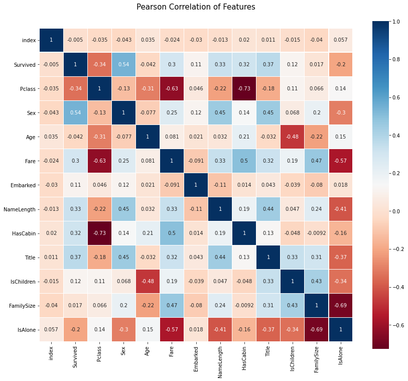
10. Feature correlation visualization
# seaborn's heatmap is used to visualize the correlation between features
colormap = plt.cm.RdBu
plt.figure(figsize=(14,12))
plt.title('Pearson Correlation of Features', y=1.05, size=15)
sns.heatmap(train_df.astype(float).corr(),linewidths=0.1,vmax=1.0,
            square=True, cmap=colormap, linecolor='white', annot=True)
plt.show()
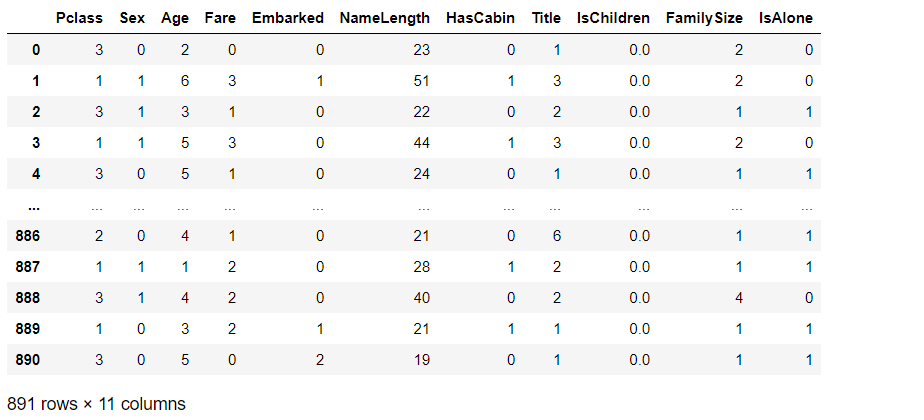
X_train = train_df.drop(['Survived','index'],axis=1)
Y_train = train_df["Survived"]
X_test = test_df.drop("PassengerId",axis=1).copy()
X_train
Y_train
X_test.head()
X_train.shape,Y_train.shape,X_test.shape

Modeling and optimization
1. Logistic regression
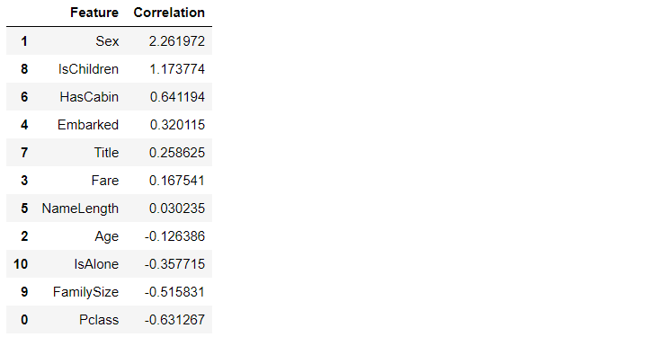
# Logistic Regression model
logreg = LogisticRegression()
logreg.fit(X_train,Y_train)
Y_pred_logreg = logreg.predict(X_test)
acc_log = round(logreg.score(X_train,Y_train)*100,2)
# Prediction results
Y_pred_logreg
acc_log

Calculate correlation
# Calculate correlation
coeff_df = pd.DataFrame(train_df.columns.delete(0))
coeff_df.columns = ['Feature']
coeff_df["Correlation"] = pd.Series(logreg.coef_[0])

coeff_df.sort_values(by='Correlation', ascending=False)
2.SVC (support vector machine)
# Support Vector Machines

svc = SVC()
svc.fit(X_train, Y_train)
Y_pred_svc = svc.predict(X_test)
acc_svc = round(svc.score(X_train, Y_train) * 100, 2)
Y_pred_svc
acc_svc

3.KNN (K-nearest neighbor classification algorithm)
# KNN k nearest neighbor classification model
knn = KNeighborsClassifier(n_neighbors = 3)
knn.fit(X_train, Y_train)
Y_pred_knn = knn.predict(X_test)
acc_knn = round(knn.score(X_train, Y_train) * 100, 2)
Y_pred_knn
acc_knn

4.GNB (Bayesian classification algorithm)
# Bayesian classification
# Gaussian Naive Bayes

gaussian = GaussianNB()
gaussian.fit(X_train, Y_train)
Y_pred_gaussian = gaussian.predict(X_test)
acc_gaussian = round(gaussian.score(X_train, Y_train) * 100, 2)
Y_pred_gaussian
acc_gaussian

5.Perceptron model
# Perceptron

perceptron = Perceptron()
perceptron.fit(X_train, Y_train)
Y_pred_perceptron = perceptron.predict(X_test)
acc_perceptron = round(perceptron.score(X_train, Y_train) * 100, 2)
acc_perceptron
acc_perceptron

6.Linear SVC
# Linear SVC

linear_svc = LinearSVC()
linear_svc.fit(X_train, Y_train)
Y_pred_linear_svc= linear_svc.predict(X_test)
acc_linear_svc = round(linear_svc.score(X_train, Y_train) * 100, 2)
Y_pred_linear_svc
acc_linear_svc

7.SGD model
# Stochastic Gradient Descent

sgd = SGDClassifier()
sgd.fit(X_train, Y_train)
Y_pred_sgd = sgd.predict(X_test)
acc_sgd = round(sgd.score(X_train, Y_train) * 100, 2)
Y_pred_sgd
acc_sgd

8. Decision tree model
# Decision Tree model

decision_tree = DecisionTreeClassifier()
decision_tree.fit(X_train, Y_train)
Y_pred_decision_tree = decision_tree.predict(X_test)
acc_decision_tree = round(decision_tree.score(X_train, Y_train) * 100, 2)
Y_pred_decision_tree
acc_decision_tree

9. Random forest algorithm
from sklearn.model_selection import train_test_split

X_all = train_df.drop(['Survived'], axis=1)
y_all = train_df['Survived']

num_test = 0.20
X_train, X_test, y_train, y_test = train_test_split(X_all, y_all, test_size=num_test, random_state=23)
# Random Forest
from sklearn.metrics import make_scorer, accuracy_score
from sklearn.model_selection import GridSearchCV
random_forest = RandomForestClassifier()
parameters = {'n_estimators': [4, 6, 9],
'max_features': ['log2', 'sqrt','auto'],
'criterion': ['entropy', 'gini'],
'max_depth': [2, 3, 5, 10],
'min_samples_split': [2, 3, 5],
'min_samples_leaf': [1,5,8]
}
acc_scorer = make_scorer(accuracy_score)
grid_obj = GridSearchCV(random_forest, parameters, scoring=acc_scorer)
grid_obj = grid_obj.fit(X_train, y_train)
clf = grid_obj.best_estimator_
clf.fit(X_train, y_train)
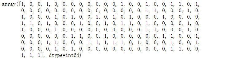
pred = clf.predict(X_test)
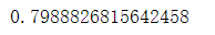
acc_random_forest_split=accuracy_score(y_test, pred)
pred
acc_random_forest_split
10.kfold cross validation model
from sklearn.model_selection import KFold
def run_kfold(clf):
kf = KFold(891,n_splits=10)
outcomes = []
fold = 0
for train_index, test_index in kf.split(train_df):
fold += 1
X_train, X_test = X_all.values[train_index], X_all.values[test_index]
y_train, y_test = y_all.values[train_index], y_all.values[test_index]
clf.fit(X_train, y_train)
predictions = clf.predict(X_test)
accuracy = accuracy_score(y_test, predictions)
outcomes.append(accuracy)
mean_outcome = np.mean(outcomes)
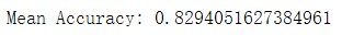
print("Mean Accuracy: {0}".format(mean_outcome))
run_kfold(clf)
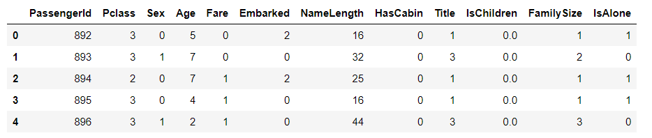
test_df.head()
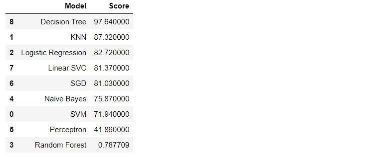
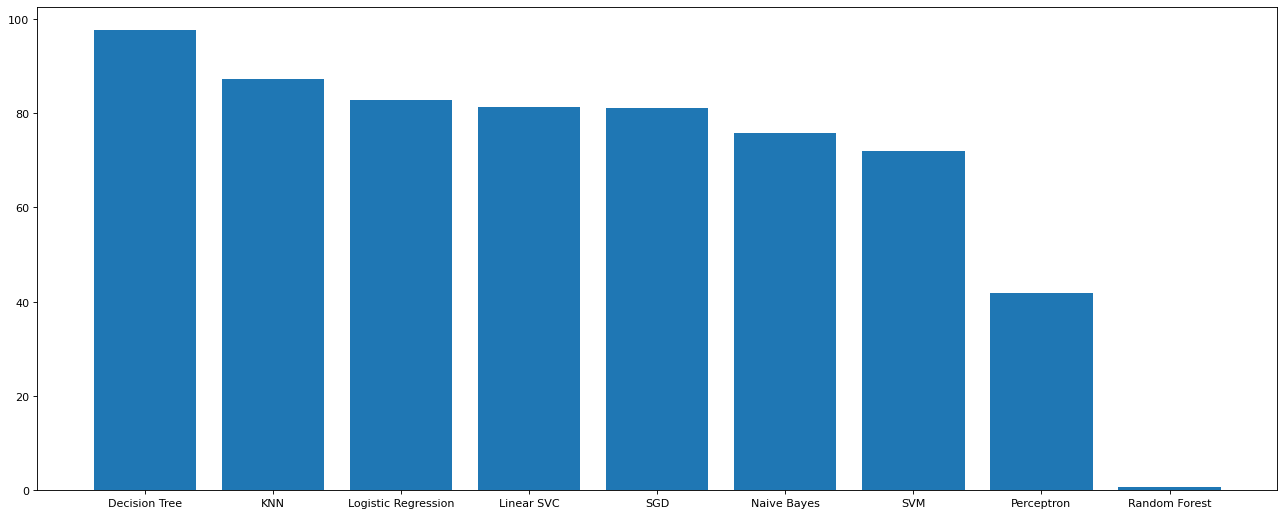
Model effect comparison
Y_pred_random_forest_split = clf.predict(test_df.drop("PassengerId",axis=1))
models = pd.DataFrame({
    'Model': ['SVM', 'KNN', 'Logistic Regression',
              'Random Forest', 'Naive Bayes', 'Perceptron',
              'SGD', 'Linear SVC',
              'Decision Tree'],
    'Score': [acc_svc, acc_knn,
              acc_log,
              acc_random_forest_split,
              #acc_random_forest,
              acc_gaussian,
              acc_perceptron,
              acc_sgd,
              acc_linear_svc,
              acc_decision_tree]})
M_s = models.sort_values(by='Score', ascending=False)
M_s
plt.figure(figsize=(20,8),dpi=80)
plt.bar(M_s['Model'],M_s['Score'])
plt.show()
Save results
# Import the time module and use the time stamp as the file name
import time
print(time.strftime('%Y%m%d%H%M',time.localtime(time.time())))

1. Save the prediction results of random forest model
# Take the prediction data of the last updated random forest model and submit it
submission = pd.DataFrame({
        "PassengerId": test_df["PassengerId"],
        "Survived": Y_pred_random_forest_split
        #"Survived": Y_pred_random_forest
    })
submission.to_csv('E:/PythonData/titanic/submission_random_forest_'
                  +time.strftime('%Y%m%d%H%M',time.localtime(time.time()))
                  +".csv",
                  index=False)
2. Save the prediction results of the decision tree model
submission = pd.DataFrame({
        "PassengerId": test_df["PassengerId"],
        "Survived": Y_pred_decision_tree
    })
submission.to_csv('E:/PythonData/titanic/submission_decision_tree'
                  +time.strftime('%Y%m%d%H%M',time.localtime(time.time()))
                  +".csv",
                  index=False)
3. Save KNN model prediction results
submission = pd.DataFrame({
        "PassengerId": test_df["PassengerId"],
        "Survived": Y_pred_knn
    })
submission.to_csv('E:/PythonData/titanic/submission_knn_'
                  +time.strftime('%Y%m%d%H%M',time.localtime(time.time()))
                  +".csv",
                  index=False)
4. Save the prediction results of SVC (support vector machine model)
submission = pd.DataFrame({
        "PassengerId": test_df["PassengerId"],
        "Survived": Y_pred_svc
    })
submission.to_csv('E:/PythonData/titanic/submission_svc_'
                  +time.strftime('%Y%m%d%H%M',time.localtime(time.time()))
                  +".csv",
                  index=False)
5. Save the prediction results of SGD model
# SGD
submission = pd.DataFrame({
        "PassengerId": test_df["PassengerId"],
        "Survived": Y_pred_sgd
    })
submission.to_csv('E:/PythonData/titanic/submission_sgd_'
                  +time.strftime('%Y%m%d%H%M',time.localtime(time.time()))
                  +".csv",
                  index=False)
6. Save the prediction results of Linear SVC model
# Linear SVC
submission = pd.DataFrame({
        "PassengerId": test_df["PassengerId"],
        "Survived": Y_pred_linear_svc
    })
submission.to_csv('E:/PythonData/titanic/submission_linear_svc_'
                  +time.strftime('%Y%m%d%H%M',time.localtime(time.time()))
                  +".csv",
                  index=False)
7. Save the prediction results of logistic regression model
# logistic regression
submission = pd.DataFrame({
        "PassengerId": test_df["PassengerId"],
        "Survived": Y_pred_logreg
    })
submission.to_csv('E:/PythonData/titanic/submission_logreg_'
                  +time.strftime('%Y%m%d%H%M',time.localtime(time.time()))
                  +".csv",
                  index=False)
Result file