Import numpy and view version
import numpy as np
np.__version__
'1.13.1'
What is numpy?
That is, Numeric Python. After expansion, python can support array and matrix types, including a large number of matrix and array calculation functions
Numpy framework is the basis of machine learning and data mining. pandas, scipy and matplotlib are all based on numpy
1, Create ndarray and view data types
The most basic data structure in numpy is ndarray: array
1. Use NP Array() is created by python list
data = [1,2,3]
nd = np.array(data)
nd
array([1, 2, 3])
type(data),type(nd)
(list, numpy.ndarray)
# View the types of elements in nd
nd.dtype
dtype('int32')
nd2 = np.array([1,3,4.6,"fdsaf",True])
nd2
array(['1', '3', '4.6', 'fdsaf', 'True'],
      dtype='<U32')
nd2.dtype
dtype('<U32')
[note]
1. All elements in the array are of the same type
2. If the array is created from a list, the element classes in the list will be unified into a certain type (priority: STR > float > int)
Relationship between image and array
# Note: pictures are also an array in numpy
# Import a picture
import matplotlib.pyplot as plt
# This tool is a data visualization analysis tool. Here I use it to import pictures
girl = plt.imread("./source/girl.jpg")
type(girl) # After the image is imported, it is an array of type array
numpy.ndarray
# View the shape of the array
girl.shape
# The shape attribute is a tuple. Each element of the tuple represents the number of elements of the array girl in this dimension
(900, 1440, 3)
girl
array([[[225, 231, 231],
        [229, 235, 235],
        [222, 228, 228],
        ...,
        [206, 213, 162],
        [211, 213, 166],
        [217, 220, 173]],

       [[224, 230, 230],
        [229, 235, 235],
        [223, 229, 229],
        ...,
        [206, 213, 162],
        [211, 213, 166],
        [217, 220, 173]],

       [[224, 230, 230],
        [229, 235, 235],
        [223, 229, 229],
        ...,
        [206, 213, 162],
        [211, 213, 166],
        [219, 221, 174]],

       ...,
       [[175, 187, 213],
        [180, 192, 218],
        [175, 187, 213],
        ...,
        [155, 162, 180],
        [153, 160, 178],
        [156, 163, 181]],

       [[175, 187, 213],
        [180, 192, 218],
        [174, 186, 212],
        ...,
        [155, 162, 180],
        [153, 160, 178],
        [155, 162, 180]],

       [[177, 189, 215],
        [181, 193, 219],
        [174, 186, 212],
        ...,
        [155, 162, 180],
        [153, 160, 178],
        [156, 163, 181]]], dtype=uint8)
# Use the plt tool to display the picture
plt.imshow(girl)
plt.show()

Create a picture
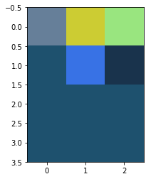
# Create a picture
boy = np.array([[[0.4,0.5,0.6],[0.8,0.8,0.2],[0.6,0.9,0.5]],
                [[0.12,0.32,0.435],[0.22,0.45,0.9],[0.1,0.2,0.3]],
                [[0.12,0.32,0.435],[0.12,0.32,0.435],[0.12,0.32,0.435]],
                [[0.12,0.32,0.435],[0.12,0.32,0.435],[0.12,0.32,0.435]]])
boy
array([[[ 0.4  ,  0.5  ,  0.6  ],
        [ 0.8  ,  0.8  ,  0.2  ],
        [ 0.6  ,  0.9  ,  0.5  ]],

       [[ 0.12 ,  0.32 ,  0.435],
        [ 0.22 ,  0.45 ,  0.9  ],
        [ 0.1  ,  0.2  ,  0.3  ]],

       [[ 0.12 ,  0.32 ,  0.435],
        [ 0.12 ,  0.32 ,  0.435],
        [ 0.12 ,  0.32 ,  0.435]],

       [[ 0.12 ,  0.32 ,  0.435],
        [ 0.12 ,  0.32 ,  0.435],
        [ 0.12 ,  0.32 ,  0.435]]])
plt.imshow(boy)
plt.show()
The two-dimensional array can also represent a picture. The two-dimensional picture is gray-scale
#The two-dimensional array can also represent a picture. The two-dimensional picture is gray-scale
boy2 = np.array([[0.1,0.2,0.3,0.4],
                 [0.6,0.3,0.2,0.5],
                 [0.9,0.8,0.3,0.2]])
boy2
array([[ 0.1,  0.2,  0.3,  0.4],
       [ 0.6,  0.3,  0.2,  0.5],
       [ 0.9,  0.8,  0.3,  0.2]])
plt.imshow(boy2,cmap="gray")
plt.show()
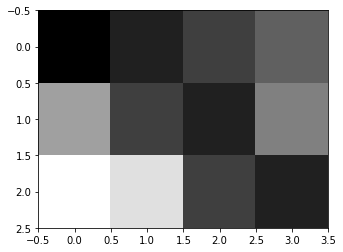
Image cutting: take out a part of the image
# Cut picture
g = girl[:200,:300]
plt.imshow(g)
plt.show()
2. Use np's common functions to create
1)np.ones(shape,dtype=None,order='C')
np.ones((2,3,3,4,5))
# The shape parameter represents the shape of the array. It is required to pass a tuple or list, and each element of the tuple
# Represents the number of elements in this dimension of the created array
array([[[[[ 1.,  1.,  1.,  1.,  1.],
          [ 1.,  1.,  1.,  1.,  1.],
          [ 1.,  1.,  1.,  1.,  1.],
          [ 1.,  1.,  1.,  1.,  1.]],

         [[ 1.,  1.,  1.,  1.,  1.],
          [ 1.,  1.,  1.,  1.,  1.],
          [ 1.,  1.,  1.,  1.,  1.],
          [ 1.,  1.,  1.,  1.,  1.]],

         [[ 1.,  1.,  1.,  1.,  1.],
          [ 1.,  1.,  1.,  1.,  1.],
          [ 1.,  1.,  1.,  1.,  1.],
          [ 1.,  1.,  1.,  1.,  1.]]],


        [[[ 1.,  1.,  1.,  1.,  1.],
          [ 1.,  1.,  1.,  1.,  1.],
          [ 1.,  1.,  1.,  1.,  1.],
          [ 1.,  1.,  1.,  1.,  1.]],

         [[ 1.,  1.,  1.,  1.,  1.],
          [ 1.,  1.,  1.,  1.,  1.],
          [ 1.,  1.,  1.,  1.,  1.],
          [ 1.,  1.,  1.,  1.,  1.]],

         [[ 1.,  1.,  1.,  1.,  1.],
          [ 1.,  1.,  1.,  1.,  1.],
          [ 1.,  1.,  1.,  1.,  1.],
          [ 1.,  1.,  1.,  1.,  1.]]]],


       [[[[ 1.,  1.,  1.,  1.,  1.],
          [ 1.,  1.,  1.,  1.,  1.],
          [ 1.,  1.,  1.,  1.,  1.],
          [ 1.,  1.,  1.,  1.,  1.]],

         [[ 1.,  1.,  1.,  1.,  1.],
          [ 1.,  1.,  1.,  1.,  1.],
          [ 1.,  1.,  1.,  1.,  1.],
          [ 1.,  1.,  1.,  1.,  1.]],

         [[ 1.,  1.,  1.,  1.,  1.],
          [ 1.,  1.,  1.,  1.,  1.],
          [ 1.,  1.,  1.,  1.,  1.],
          [ 1.,  1.,  1.,  1.,  1.]]],


        [[[ 1.,  1.,  1.,  1.,  1.],
          [ 1.,  1.,  1.,  1.,  1.],
          [ 1.,  1.,  1.,  1.,  1.],
          [ 1.,  1.,  1.,  1.,  1.]],

         [[ 1.,  1.,  1.,  1.,  1.],
          [ 1.,  1.,  1.,  1.,  1.],
          [ 1.,  1.,  1.,  1.,  1.],
          [ 1.,  1.,  1.,  1.,  1.]],

         [[ 1.,  1.,  1.,  1.,  1.],
          [ 1.,  1.,  1.,  1.,  1.],
          [ 1.,  1.,  1.,  1.,  1.],
          [ 1.,  1.,  1.,  1.,  1.]]]]])
ones = np.ones((168,233,3))
plt.imshow(ones)
plt.show()
2)np.zeros(shape,dtype="float",order="C")
np.zeros((1,2,3))
array([[[ 0.,  0.,  0.],
        [ 0.,  0.,  0.]]])
3)np.full(shape,fill_value,dtype=None)
np.full((2,3),12)
array([[12, 12, 12],
       [12, 12, 12]])
4)np.eye(N,M,k=0,dtype='float')
np.eye(6)
array([[ 1.,  0.,  0.,  0.,  0.,  0.],
       [ 0.,  1.,  0.,  0.,  0.,  0.],
       [ 0.,  0.,  1.,  0.,  0.,  0.],
       [ 0.,  0.,  0.,  1.,  0.,  0.],
       [ 0.,  0.,  0.,  0.,  1.,  0.],
       [ 0.,  0.,  0.,  0.,  0.,  1.]])
np.eye(3,4)
array([[ 1.,  0.,  0.,  0.],
       [ 0.,  1.,  0.,  0.],
       [ 0.,  0.,  1.,  0.]])
np.eye(5,4)
array([[ 1.,  0.,  0.,  0.],
       [ 0.,  1.,  0.,  0.],
       [ 0.,  0.,  1.,  0.],
       [ 0.,  0.,  0.,  1.],
       [ 0.,  0.,  0.,  0.]])
5)np.linspace(start,stop,num=50)
np.linspace(1,10,num=100)
# From start to stop, divide it into num parts on average, and take the cutting point
array([  1.        ,   1.09090909,   1.18181818,   1.27272727,
         1.36363636,   1.45454545,   1.54545455,   1.63636364,
         1.72727273,   1.81818182,   1.90909091,   2.        ,
         2.09090909,   2.18181818,   2.27272727,   2.36363636,
         2.45454545,   2.54545455,   2.63636364,   2.72727273,
         2.81818182,   2.90909091,   3.        ,   3.09090909,
         3.18181818,   3.27272727,   3.36363636,   3.45454545,
         3.54545455,   3.63636364,   3.72727273,   3.81818182,
         3.90909091,   4.        ,   4.09090909,   4.18181818,
         4.27272727,   4.36363636,   4.45454545,   4.54545455,
         4.63636364,   4.72727273,   4.81818182,   4.90909091,
         5.        ,   5.09090909,   5.18181818,   5.27272727,
         5.36363636,   5.45454545,   5.54545455,   5.63636364,
         5.72727273,   5.81818182,   5.90909091,   6.        ,
         6.09090909,   6.18181818,   6.27272727,   6.36363636,
         6.45454545,   6.54545455,   6.63636364,   6.72727273,
         6.81818182,   6.90909091,   7.        ,   7.09090909,
         7.18181818,   7.27272727,   7.36363636,   7.45454545,
         7.54545455,   7.63636364,   7.72727273,   7.81818182,
         7.90909091,   8.        ,   8.09090909,   8.18181818,
         8.27272727,   8.36363636,   8.45454545,   8.54545455,
         8.63636364,   8.72727273,   8.81818182,   8.90909091,
         9.        ,   9.09090909,   9.18181818,   9.27272727,
         9.36363636,   9.45454545,   9.54545455,   9.63636364,
         9.72727273,   9.81818182,   9.90909091,  10.        ])
np.logspace(1,10,num=10)
# Divide from 1-10 into 10 parts (corresponding to 1, 2, 3... 10 respectively)
# Logx = 1 logx = 2 logx = 3 = > return values 10 ^ 1, 10 ^ 2 10^10
array([  1.00000000e+01,   1.00000000e+02,   1.00000000e+03,
         1.00000000e+04,   1.00000000e+05,   1.00000000e+06,
         1.00000000e+07,   1.00000000e+08,   1.00000000e+09,
         1.00000000e+10])
6)np. Range ([start,] stop, [step,] dtype = none) "[]" is optional
np.arange(10)
array([0, 1, 2, 3, 4, 5, 6, 7, 8, 9])
np.arange(2,12)
array([ 2, 3, 4, 5, 6, 7, 8, 9, 10, 11])
np.arange(2,12,2)
array([ 2, 4, 6, 8, 10])
7)np.random.randint(low,high=None,size=None,dtype='I')
np.random.randint(3,10,size=(10,10,3))
# Randomly generated integer array
array([[[4, 6, 6],
        [5, 9, 4],
        [5, 9, 6],
        [4, 6, 4],
        [7, 4, 9],
        [5, 9, 4],
        [8, 6, 3],
        [7, 5, 8],
        [8, 3, 4],
        [5, 4, 8]],

       [[6, 5, 8],
        [9, 3, 5],
        [8, 4, 4],
        [5, 9, 8],
        [8, 5, 6],
        [9, 4, 6],
        [5, 8, 8],
        [5, 7, 6],
        [3, 7, 9],
        [5, 5, 7]],

       [[4, 7, 5],
        [9, 4, 9],
        [3, 3, 4],
        [8, 4, 8],
        [3, 6, 3],
        [4, 4, 3],
        [4, 4, 5],
        [5, 5, 4],
        [5, 7, 9],
        [4, 4, 9]],

       [[6, 3, 8],
        [5, 9, 6],
        [5, 6, 7],
        [3, 8, 6],
        [3, 7, 8],
        [6, 9, 7],
        [6, 7, 3],
        [7, 5, 4],
        [3, 3, 6],
        [9, 9, 7]],

       [[3, 5, 6],
        [7, 4, 6],
        [5, 3, 7],
        [3, 6, 3],
        [8, 3, 8],
        [7, 9, 7],
        [8, 7, 9],
        [4, 7, 5],
        [8, 8, 6],
        [4, 5, 4]],

       [[4, 4, 9],
        [9, 8, 7],
        [6, 6, 6],
        [4, 9, 5],
        [6, 9, 6],
        [9, 4, 8],
        [4, 7, 9],
        [9, 4, 9],
        [6, 9, 3],
        [8, 5, 9]],

       [[7, 6, 3],
        [4, 5, 4],
        [5, 6, 7],
        [7, 3, 4],
        [7, 4, 8],
        [7, 5, 6],
        [4, 9, 9],
        [4, 4, 8],
        [9, 3, 6],
        [3, 6, 9]],

       [[7, 7, 4],
        [8, 6, 3],
        [3, 8, 7],
        [5, 6, 9],
        [5, 8, 4],
        [9, 4, 4],
        [3, 6, 6],
        [6, 7, 4],
        [4, 8, 8],
        [4, 6, 3]],

       [[7, 4, 9],
        [5, 3, 7],
        [5, 9, 4],
        [5, 7, 9],
        [7, 6, 6],
        [6, 3, 3],
        [9, 4, 4],
        [5, 3, 4],
        [5, 7, 9],
        [3, 3, 5]],

       [[7, 3, 8],
        [7, 6, 8],
        [5, 7, 4],
        [4, 4, 7],
        [4, 5, 9],
        [8, 3, 5],
        [5, 9, 9],
        [6, 3, 7],
        [9, 5, 7],
        [8, 5, 9]]])
8)np.random.randn(d0,d1,...,dn)
An array is generated from the first dimension to the nth dimension, and the numbers in the array conform to the standard normal distribution
np.random.randn(2,3,10)
# N(0,1)
array([[[-0.03414751, -1.01771263,  1.12067965, -0.43953023, -1.82364645,
         -0.0971702 , -0.65734554, -0.10303229,  1.52904104, -0.48624526],
        [-0.29295679, -1.09430988,  0.07499788,  0.31664607,  0.3500672 ,
         -0.18508775,  1.75620537,  0.71531162,  0.6161491 , -1.22053836],
        [ 0.7323965 ,  0.20671506, -0.58314419, -0.16540522, -0.23903187,
          1.27785655,  0.26691062, -1.45973265, -0.27273178, -1.02878312]],

       [[ 0.07655004, -0.35616184, -0.46353849, -1.8515281 , -0.26543777,
          0.76412627,  0.83337437,  0.04521198, -2.10686009,  0.84883742],
        [ 0.22188875,  0.63737544,  0.26173337, -0.11475485, -1.30431707,
          1.25062924,  2.03032414,  0.13742253, -0.98713219,  1.19711129],
        [ 0.69212245,  0.70550039, -1.15995398, -0.95507681, -0.39439139,
          2.76551965,  0.56088858,  0.54709151,  1.17615801,  0.17744971]]])
9)np.random.normal(loc=0.0,scale=1.0,size=None)
np.random.normal(175,20,size=100)
# Obey N(175,20) to generate 10 pieces of data
array([ 174.44281329,  177.66402876,  162.76426831,  210.11244283,
        161.26671985,  209.52372115,  159.92703726,  197.83048917,
        190.60230978,  170.27114821,  202.67422923,  203.04492988,
        171.13235245,  175.64710565,  200.40533303,  207.930948  ,
        141.09792492,  158.87495159,  176.74197674,  164.57884322,
        181.22386631,  156.26287142,  133.37408465,  178.07588597,
        187.50842048,  186.35236779,  153.61560634,  145.53831704,
        232.55949685,  142.01340562,  195.22465693,  188.922162  ,
        170.02159668,  167.74728882,  173.27258287,  187.68132279,
        217.7260755 ,  158.28833839,  155.11568289,  200.26945864,
        178.91552559,  149.21007505,  200.6454259 ,  169.37529856,
        201.18878627,  184.37773296,  196.67909536,  144.10223051,
        184.63682023,  167.86858875,  191.08394709,  169.98017168,
        204.05198975,  199.65286793,  176.22452948,  181.17515804,
        178.81440955,  176.79845708,  189.50950157,  136.05787608,
        199.35198398,  162.43654974,  155.61396415,  172.22147069,
        181.91161368,  192.82571507,  203.70689642,  190.79312957,
        204.48924027,  180.48880551,  176.81359193,  145.87844077,
        190.13853094,  160.22281705,  200.04783678,  165.19927728,
        184.10218694,  178.27524256,  191.58148162,  141.4792985 ,
        208.4723939 ,  163.70082179,  142.70675324,  189.25398816,
        183.53849685,  150.86998696,  172.04187127,  207.12343336,
        190.10648007,  188.18995666,  175.43040298,  183.79396855,
        172.60260342,  195.1083776 ,  194.70719705,  163.10904061,
        146.78089275,  195.2271401 ,  201.60339544,  164.91176955])
10)np.random.random(size=None)
np.random.random(size=(12,1)) # Floating point number between 0 and 1
array([[ 0.54080763],
       [ 0.95618258],
       [ 0.19457156],
       [ 0.12198452],
       [ 0.3423529 ],
       [ 0.01716331],
       [ 0.28061005],
       [ 0.51960339],
       [ 0.60122982],
       [ 0.26462352],
       [ 0.85645091],
       [ 0.32352418]])
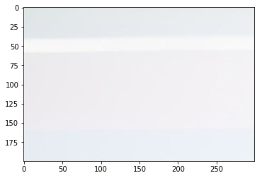
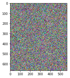
Exercise: generate a picture with random numbers
boy = np.random.random(size=(667,568,3))
plt.imshow(boy)
plt.show()
2, Common properties of ndarray
Common properties of array:
Dimension ndim, size, shape, element type dtype, size of each item itemsize, data
tigger = plt.imread("./source/tigger.jpg")
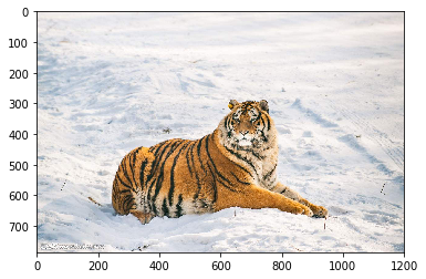
# 1. Dimensions
tigger.ndim
3
# 2. Size refers to the number of numbers in an array
tigger.size
2829600
# 3. Shape
tigger.shape
(786, 1200, 3)
# 4. Type of data
tigger.dtype
dtype('uint8')
# 5. Size of each number (in bytes)
tigger.itemsize
1
t = tigger / 255.0
t.dtype
dtype('float64')
t.itemsize
8
# 6,data
tigger.data
<memory at 0x000001AA3A0D8138>
3, Basic operation of ndarray
1. Index
l = [1,2,3,4,5,6]
l[5]
l[-1]
l[0]
l[-6]
# Positive counting starts from 0 and reverse counting starts from - 1
1
nd = np.random.randint(0,10,size=(4))
nd
array([9, 6, 1, 7])
nd[0]
nd[1]
nd[-3]
6
lp = [[1,2,3],
      [4,5,6],
      [7,8]]
lp[1][2]
6
np.array(lp)
array([list([1, 2, 3]), list([4, 5, 6]), list([7, 8])], dtype=object)
np.array(lp)
# If the value of a dimension in the two-dimensional list is inconsistent, the dimension will be packaged into a list
# [note] the number of elements of each dimension in the array must be the same
array([list([1, 2, 3]), list([4, 5, 6]), list([7, 8])], dtype=object)
nd = np.random.randint(0,10,size=(4,4))
nd
#[[2,2,1],[1,2,1]]
array([[7, 9, 2, 3],
       [0, 2, 7, 3],
       [1, 9, 0, 1],
       [4, 1, 2, 8]])
nd[1][3]
# Multiple indexing: first find the front dimension to get the sub array, and then continue indexing from the obtained sub array
3
Different from list
nd[1,3]
# Primary index: find it directly in the order of (1,3)
3
lp[1,3] # The list cannot be found like this
---------------------------------------------------------------------------

TypeError                                 Traceback (most recent call last)

<ipython-input-64-8b65614beafa> in <module>()
----> 1 lp[1,3] # The list cannot be found like this


TypeError: list indices must be integers or slices, not tuple
nd[[1,1,2,3,1,2]]
# Index with list: traverse the array in the order specified in the list
array([[0, 2, 7, 3],
       [0, 2, 7, 3],
       [1, 9, 0, 1],
       [4, 1, 2, 8],
       [0, 2, 7, 3],
       [1, 9, 0, 1]])
lp[[1,1]] # The index of a list cannot be a list
---------------------------------------------------------------------------

TypeError                                 Traceback (most recent call last)

<ipython-input-66-e9ca25f0b661> in <module>()
----> 1 lp[[1,1]] # The index of a list cannot be a list


TypeError: list indices must be integers or slices, not list
nd[[1,2,2,2]][[0,1,2]]
array([[0, 2, 7, 3],
       [1, 9, 0, 1],
       [1, 9, 0, 1]])
nd[[2,2,1]]
array([[1, 9, 0, 1],
       [1, 9, 0, 1],
       [0, 2, 7, 3]])
nd[[2,2,1,1],[1,2,1,1]]
array([9, 0, 2, 2])
2. Slice
nd
array([[7, 9, 2, 3],
       [0, 2, 7, 3],
       [1, 9, 0, 1],
       [4, 1, 2, 8]])
nd[0:100] # The right side of an interval that is closed on the left and open on the right can be infinite
array([[7, 9, 2, 3],
       [0, 2, 7, 3],
       [1, 9, 0, 1],
       [4, 1, 2, 8]])
lp[0:100]
[[1, 2, 3], [4, 5, 6], [7, 8]]
nd[:2]
array([[7, 9, 2, 3],
       [0, 2, 7, 3]])
nd[1:]
array([[0, 2, 7, 3],
       [1, 9, 0, 1],
       [4, 1, 2, 8]])
nd[3:0:-1]
# If the step length is negative, it represents the number from back to front, and the required interval is also reversed
array([[4, 1, 2, 8],
       [1, 9, 0, 1],
       [0, 2, 7, 3]])
nd
array([[7, 9, 2, 3],
       [0, 2, 7, 3],
       [1, 9, 0, 1],
       [4, 1, 2, 8]])
nd[:,0::2]
array([[7, 2],
       [0, 7],
       [1, 0],
       [4, 2]])
nd[1:3,0:2] # Cut rows and columns
array([[0, 2],
       [1, 9]])
Turn girl upside down
girl
array([[[225, 231, 231],
        [229, 235, 235],
        [222, 228, 228],
        ...,
        [206, 213, 162],
        [211, 213, 166],
        [217, 220, 173]],

       [[224, 230, 230],
        [229, 235, 235],
        [223, 229, 229],
        ...,
        [206, 213, 162],
        [211, 213, 166],
        [217, 220, 173]],

       [[224, 230, 230],
        [229, 235, 235],
        [223, 229, 229],
        ...,
        [206, 213, 162],
        [211, 213, 166],
        [219, 221, 174]],

       ...,
       [[175, 187, 213],
        [180, 192, 218],
        [175, 187, 213],
        ...,
        [155, 162, 180],
        [153, 160, 178],
        [156, 163, 181]],

       [[175, 187, 213],
        [180, 192, 218],
        [174, 186, 212],
        ...,
        [155, 162, 180],
        [153, 160, 178],
        [155, 162, 180]],

       [[177, 189, 215],
        [181, 193, 219],
        [174, 186, 212],
        ...,
        [155, 162, 180],
        [153, 160, 178],
        [156, 163, 181]]], dtype=uint8)
plt.imshow(girl[::-2,::-2])
plt.show()

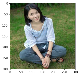
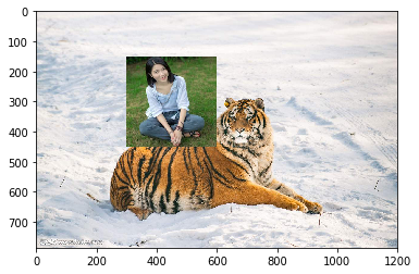
Jigsaw puzzle: put the girl on the tiger's back
t = tigger.copy() #
plt.imshow(tigger)
plt.show()

girl2 = plt.imread("./source/girl2.jpg")
plt.imshow(girl2)
plt.show()
# Dig a hole for a tiger
tigger[150:450,300:600] = girl2
plt.imshow(tigger)
plt.show()
3. Deformation
reshape()
resize()
tigger.shape
(786, 1200, 3)
nd = np.random.randint(0,10,size=12)
nd
array([4, 0, 1, 1, 8, 7, 7, 5, 3, 0, 7, 3])
nd.shape
(12,)
nd.reshape((3,2,2,1)) # The parameter is a tuple, which represents the shape of nd
array([[[[4],
         [0]],

        [[1],
         [1]]],


       [[[8],
         [7]],

        [[7],
         [5]]],


       [[[3],
         [0]],

        [[7],
         [3]]]])
nd
array([4, 0, 1, 1, 8, 7, 7, 5, 3, 0, 7, 3])
nd.reshape((3,2))#cannot reshape array of size 12 into shape (3,8)
# Keep consistent when deforming
---------------------------------------------------------------------------

ValueError                                Traceback (most recent call last)

<ipython-input-94-dda3397392b8> in <module>()
----> 1 nd.reshape((3,2))#cannot reshape array of size 12 into shape (3,8)


ValueError: cannot reshape array of size 12 into shape (3,2)
nd.resize((2,6))
nd
array([[4, 0, 1, 1, 8, 7],
       [7, 5, 3, 0, 7, 3]])
[note]
  1)Of arrays before and after deformation size Be consistent, or you can't deform
  2)reshape()The function is to copy the original array, deform the copy, and return the deformation result
  3)resize()The function deforms the original array and does not need to return the result
4. Cascade
Cascade: it is to connect two arrays according to the specified dimension
nd1 = np.random.randint(0,10,size=(4,4))
nd2 = np.random.randint(20,40,size=(3,4))
print(nd1)
print(nd2)
[[2 5 6 1]
 [4 8 0 5]
 [9 4 7 8]
 [4 3 0 8]]
[[38 22 25 38]
 [22 38 30 21]
 [23 34 28 26]]
# Concatenate two arrays
np.concatenate([nd1,nd2],axis=0)
# Parameter 1 is a list (or tuple), which contains the arrays involved in the cascade
# The parameter axis defaults to 0, which means cascading on the row (the 0th dimension), and 1, which means cascading on the column (the 1st dimension)
array([[ 2,  5,  6,  1],
       [ 4,  8,  0,  5],
       [ 9,  4,  7,  8],
       [ 4,  3,  0,  8],
       [38, 22, 25, 38],
       [22, 38, 30, 21],
       [23, 34, 28, 26]])
np.concatenate([nd1,nd2],axis=1)
# Column concatenation requires the same number of rows
---------------------------------------------------------------------------

ValueError                                Traceback (most recent call last)

<ipython-input-102-0a76346b819d> in <module>()
----> 1 np.concatenate([nd1,nd2],axis=1)


ValueError: all the input array dimensions except for the concatenation axis must match exactly
nd3 = np.random.randint(0,10,size=(4,3))
nd3
array([[1, 3, 7],
       [9, 5, 3],
       [9, 0, 2],
       [0, 7, 4]])
nd1
array([[2, 5, 6, 1],
       [4, 8, 0, 5],
       [9, 4, 7, 8],
       [4, 3, 0, 8]])
np.concatenate([nd1,nd3])
# The number of columns is inconsistent. Row concatenation is not allowed
---------------------------------------------------------------------------

ValueError                                Traceback (most recent call last)

<ipython-input-106-871caaeeb895> in <module>()
----> 1 np.concatenate([nd1,nd3])


ValueError: all the input array dimensions except for the concatenation axis must match exactly
np.concatenate([nd1,nd3],axis=1)
array([[2, 5, 6, 1, 1, 3, 7],
       [4, 8, 0, 5, 9, 5, 3],
       [9, 4, 7, 8, 9, 0, 2],
       [4, 3, 0, 8, 0, 7, 4]])
extension
1) Only when the shape is consistent can it be cascaded
nd4 = np.random.randint(0,10,size=(1,2,3))
nd5 = np.random.randint(0,10,size=(1,4,3))
print(nd4)
print(nd5)
[[[2 9 8]
  [9 5 6]]]
[[[9 9 6]
  [8 3 4]
  [8 7 7]
  [0 6 6]]]
np.concatenate([nd4,nd5],axis=1)
array([[[2, 9, 8],
        [9, 5, 6],
        [9, 9, 6],
        [8, 3, 4],
        [8, 7, 7],
        [0, 6, 6]]])
nd6 = np.random.randint(0,10,size=4)
nd6
array([3, 5, 3, 6])
2) Dimension inconsistency cannot be cascaded
np.concatenate([nd1,nd6])
---------------------------------------------------------------------------

ValueError                                Traceback (most recent call last)

<ipython-input-124-6dd6213f71bc> in <module>()
----> 1 np.concatenate([nd1,nd6])


ValueError: all the input arrays must have same number of dimensions
Problems needing attention in cascading:
1)Dimensions must be the same
2)The shape must match( axis Equal to which dimension. After we remove this dimension, the remaining shapes must be consistent)
3)The cascade direction can have axis To specify, the default is 0
hstack and vstack are also available for two-dimensional arrays
nd = np.random.randint(0,10,size=(10,1))
nd
array([[1],
       [7],
       [6],
       [9],
       [0],
       [4],
       [6],
       [2],
       [0],
       [8]])
np.hstack(nd)
array([1, 7, 6, 9, 0, 4, 6, 2, 0, 8])
nd1 = np.random.randint(0,10,size=(10,2))
nd1
array([[4, 4],
       [3, 1],
       [3, 3],
       [9, 6],
       [5, 1],
       [4, 7],
       [3, 3],
       [4, 3],
       [7, 9],
       [6, 5]])
np.hstack(nd1)
array([4, 4, 3, 1, 3, 3, 9, 6, 5, 1, 4, 7, 3, 3, 4, 3, 7, 9, 6, 5])
np.vstack(nd1)
array([[4, 4],
       [3, 1],
       [3, 3],
       [9, 6],
       [5, 1],
       [4, 7],
       [3, 3],
       [4, 3],
       [7, 9],
       [6, 5]])
nd2 = np.random.randint(0,10,size=10)
nd2
array([1, 7, 4, 3, 9, 0, 3, 3, 2, 5])
np.vstack(nd2)
array([[1],
       [7],
       [4],
       [3],
       [9],
       [0],
       [3],
       [3],
       [2],
       [5]])
np.hstack(nd2)
array([1, 7, 4, 3, 9, 0, 3, 3, 2, 5])
hstack() changes a column array to a row array and a two-dimensional array to a one-dimensional array
vstack() changes the row array to the column array, and changes the one-dimensional array to two-dimensional (takes each element in the one-dimensional array as a row)
5. Segmentation
Slicing is to cut an array into multiple
vsplit()
hsplit()
split()
nd = np.random.randint(0,100,size=(5,6))
nd
array([[17, 47, 83, 33, 69, 24],
       [60,  4, 34, 29, 75, 60],
       [33, 55, 67,  1, 76, 82],
       [31, 92,  1, 14, 83, 95],
       [59, 88, 81, 49, 70, 11]])
# Horizontal segmentation
np.hsplit(nd,[1,4,5,8,9])
# Parameter 1 represents the array to be segmented, and parameter 2 is a list representing the location of the segmentation point
[array([[17],
        [60],
        [33],
        [31],
        [59]]), array([[47, 83, 33],
        [ 4, 34, 29],
        [55, 67,  1],
        [92,  1, 14],
        [88, 81, 49]]), array([[69],
        [75],
        [76],
        [83],
        [70]]), array([[24],
        [60],
        [82],
        [95],
        [11]]), array([], shape=(5, 0), dtype=int32), array([], shape=(5, 0), dtype=int32)]
# Vertical segmentation
np.vsplit(nd,[1,3,5])
[array([[17, 47, 83, 33, 69, 24]]), array([[60,  4, 34, 29, 75, 60],
        [33, 55, 67,  1, 76, 82]]), array([[31, 92,  1, 14, 83, 95],
        [59, 88, 81, 49, 70, 11]]), array([], shape=(0, 6), dtype=int32)]
split() function
nd
array([[17, 47, 83, 33, 69, 24],
       [60,  4, 34, 29, 75, 60],
       [33, 55, 67,  1, 76, 82],
       [31, 92,  1, 14, 83, 95],
       [59, 88, 81, 49, 70, 11]])
np.split(nd,[1,2],axis=0)
# The default value of axis is 0, which means cutting on the 0th dimension, and 1 means cutting on the 1st dimension
[array([[17, 47, 83, 33, 69, 24]]),
 array([[60,  4, 34, 29, 75, 60]]),
 array([[33, 55, 67,  1, 76, 82],
        [31, 92,  1, 14, 83, 95],
        [59, 88, 81, 49, 70, 11]])]
extension
nd1 = np.random.randint(0,10,size=(3,4,5))
nd1
array([[[5, 7, 8, 7, 9],
        [3, 6, 1, 9, 0],
        [6, 0, 2, 6, 9],
        [4, 5, 5, 3, 9]],

       [[6, 7, 6, 2, 3],
        [3, 0, 0, 5, 3],
        [9, 9, 0, 6, 2],
        [5, 4, 5, 4, 4]],

       [[8, 7, 4, 8, 9],
        [2, 2, 1, 7, 3],
        [2, 2, 9, 4, 7],
        [7, 3, 9, 4, 1]]])
np.split(nd1,[2],axis=2)
[array([[[5, 7],
         [3, 6],
         [6, 0],
         [4, 5]],

        [[6, 7],
         [3, 0],
         [9, 9],
         [5, 4]],

        [[8, 7],
         [2, 2],
         [2, 2],
         [7, 3]]]), array([[[8, 7, 9],
         [1, 9, 0],
         [2, 6, 9],
         [5, 3, 9]],

        [[6, 2, 3],
         [0, 5, 3],
         [0, 6, 2],
         [5, 4, 4]],

        [[4, 8, 9],
         [1, 7, 3],
         [9, 4, 7],
         [9, 4, 1]]])]
6. Copy
nd = np.random.randint(0,100,size=6)
nd
array([34, 69, 14, 2, 48, 74])
nd1 = nd
# The assignment between arrays is only a copy of the address, and the array object itself is not copied
nd1
array([34, 69, 14, 2, 48, 74])
nd1[0] = 100
nd1
array([100, 69, 14, 2, 48, 74])
nd
array([100, 69, 14, 2, 48, 74])
nd2 = nd.copy()
# The copy function copies a copy of the array referenced by nd, and stores the address of the copy in nd2
nd2[0] = 200000
nd
array([100, 69, 14, 2, 48, 74])
nd1
array([100, 69, 14, 2, 48, 74])
nd2
array([200000, 69, 14, 2, 48, 74])
Discussion: the process of creating an array from a list includes the creation of a copy
l = [1,2,3]
l
[1, 2, 3]
nd = np.array(l)
nd
array([1, 2, 3])
nd[0] = 1000
l
[1, 2, 3]
Note: the process of creating an array from a list is to copy a copy of the list, then unify the element types in the copy, and then put them into the array object
4, Aggregation operation of ndarray
Aggregation operation refers to solving some characteristics of the data in the array
1. Sum
nd = np.random.randint(0,10,size=(3,4))
nd
array([[5, 9, 6, 8],
       [3, 7, 1, 9],
       [5, 7, 6, 3]])
nd.sum() # Complete aggregation
69
nd.sum(axis=0) # Aggregate rows (that is, aggregate dimension 0)
array([13, 23, 13, 20])
nd.sum(axis=1) # Aggregate columns (that is, aggregate the first dimension)
array([28, 20, 21])
extension
nd = np.random.randint(0,10,size=(2,3,4))
nd
array([[[1, 0, 0, 3],
        [9, 6, 1, 8],
        [4, 9, 3, 9]],

       [[8, 0, 4, 3],
        [3, 0, 1, 8],
        [8, 0, 7, 4]]])
nd.sum()
99
nd.sum(axis=0)
array([[ 9,  0,  4,  6],
       [12,  6,  2, 16],
       [12,  9, 10, 13]])
nd.sum(axis=2)
array([[ 4, 24, 25],
       [15, 12, 19]])
Rule of aggregation operation: change the aggregation axis through axis. When axis=x, the X dimension will disappear and the corresponding elements in this dimension will be aggregated
Exercise: given a 4-dimensional matrix, how to get the sum of the last two dimensions?
nd1 = np.random.randint(0,10,size=(2,3,4,5))
nd1
array([[[[3, 2, 9, 4, 0],
         [1, 0, 2, 3, 7],
         [4, 8, 6, 6, 5],
         [2, 3, 4, 1, 5]],

        [[3, 2, 0, 1, 3],
         [7, 3, 3, 4, 1],
         [0, 4, 0, 6, 9],
         [3, 8, 6, 0, 5]],

        [[5, 1, 3, 5, 0],
         [1, 4, 1, 8, 0],
         [9, 1, 9, 6, 5],
         [6, 1, 8, 5, 1]]],


       [[[7, 5, 3, 4, 5],
         [7, 8, 6, 7, 2],
         [9, 9, 5, 3, 4],
         [9, 2, 9, 7, 2]],

        [[3, 2, 9, 7, 7],
         [0, 8, 1, 3, 0],
         [1, 5, 5, 6, 5],
         [4, 8, 7, 2, 9]],

        [[1, 3, 5, 0, 6],
         [6, 0, 3, 5, 6],
         [2, 4, 6, 9, 0],
         [8, 7, 4, 0, 6]]]])
Writing method I
nd1.sum(axis=2).sum(axis=2)
array([[ 75,  68,  79],
       [113,  92,  81]])
Writing method 2
nd1.sum(axis=-1).sum(axis=-1)
array([[ 75,  68,  79],
       [113,  92,  81]])
Writing method III
nd1.sum(axis=(-1,-2))
array([[ 75,  68,  79],
       [113,  92,  81]])
2. Maximum value
nd
array([[[1, 0, 0, 3],
        [9, 6, 1, 8],
        [4, 9, 3, 9]],

       [[8, 0, 4, 3],
        [3, 0, 1, 8],
        [8, 0, 7, 4]]])
nd.sum(axis=-1)
array([[ 4, 24, 25],
       [15, 12, 19]])
nd.max()
9
nd.max(axis=-1)
array([[3, 9, 9],
       [8, 8, 8]])
nd.max(axis=1)
array([[9, 9, 3, 9],
       [8, 0, 7, 8]])
nd.min(axis=0)
array([[1, 0, 0, 3],
       [3, 0, 1, 8],
       [4, 0, 3, 4]])
3. Other aggregation operations
Function Name	NaN-safe Version	Description
np.sum	np.nansum	Compute sum of elements
np.prod	np.nanprod	Compute product of elements
np.mean	np.nanmean	Compute mean of elements
np.std	np.nanstd	Compute standard deviation
np.var	np.nanvar	Compute variance
np.min	np.nanmin	Find minimum value
np.max	np.nanmax	Find maximum value
np.argmin	np.nanargmin	Find index of minimum value
np.argmax	np.nanargmax	Find index of maximum value
np.median	np.nanmedian	Compute median of elements
np.percentile	np.nanpercentile	Compute rank-based statistics of elements
np.any	N/A	Evaluate whether any elements are true
np.all	N/A	Evaluate whether all elements are true
np.power exponentiation
np.nan
# This number represents missing and defaults to floating point type
type(np.nan) # Any number and nan operations are missing
float
np.nan + 10
nan
np.nan*10
nan
nd2 = np.array([12,23,np.nan,34,np.nan,90])
nd2
array([ 12., 23., nan, 34., nan, 90.])
# Polymerization of nd2
nd2.sum(axis=0)
nan
nd2.max()
nan
Normal aggregation will cause interference to the missing array, so we need to use aggregation with nan
np.nansum(nd2)
159.0
np.nanmean(nd2)
39.75
Aggregation operation:
1)axis Specifies the dimension of aggregation. By default, it does not represent complete aggregation (that is, aggregate all arrays to get a constant). If axis Value specifies which dimension, and this dimension will disappear and be replaced by the results after aggregation
2)numpy There are two versions of the aggregate function nan And without nan,belt nan The missing items will be directly eliminated during aggregation
Thinking question: how to sort a 5 * 5 matrix according to column 3?
nd = np.random.randint(0,100,size=(5,5))
nd
array([[70, 76, 87, 23, 68],
       [34,  3, 59, 93, 71],
       [71, 64, 98, 31, 70],
       [59, 17, 71, 99, 50],
       [86, 58, 91, 22, 18]])
sort
np.sort(nd,axis=0)
array([[34,  3, 59, 22, 18],
       [59, 17, 71, 23, 50],
       [70, 58, 87, 31, 68],
       [71, 64, 91, 93, 70],
       [86, 76, 98, 99, 71]])
np.sort(nd[:,3])
array([22, 23, 31, 93, 99])
nd[[4,0,2,1,3]]
array([[86, 58, 91, 22, 18],
       [70, 76, 87, 23, 68],
       [71, 64, 98, 31, 70],
       [34,  3, 59, 93, 71],
       [59, 17, 71, 99, 50]])
ind = np.argsort(nd[:,3]) # After sorting from small to large, the subscript corresponding to the element is returned
ind
array([4, 0, 2, 1, 3], dtype=int64)
nd[ind]
array([[86, 58, 91, 22, 18],
       [70, 76, 87, 23, 68],
       [71, 64, 98, 31, 70],
       [34,  3, 59, 93, 71],
       [59, 17, 71, 99, 50]])
5, Matrix operation of ndarray
1. Basic matrix operation
1) Arithmetic operation (i.e. addition, subtraction, multiplication and division)
nd = np.random.randint(0,10,size=(3,3))
nd
array([[7, 4, 6],
       [4, 5, 1],
       [0, 2, 5]])
nd + nd
array([[14,  8, 12],
       [ 8, 10,  2],
       [ 0,  4, 10]])
nd + 2 # Here, the constant 2 will be amplified into a 3 * 3 matrix with all values of 2
array([[9, 6, 8],
       [6, 7, 3],
       [2, 4, 7]])
nd - 2
array([[ 5,  2,  4],
       [ 2,  3, -1],
       [-2,  0,  3]])
In mathematics, a matrix can be multiplied by or divided by a constant
nd * 4
array([[28, 16, 24],
       [16, 20,  4],
       [ 0,  8, 20]])
nd / 4
array([[ 1.75,  1.  ,  1.5 ],
       [ 1.  ,  1.25,  0.25],
       [ 0.  ,  0.5 ,  1.25]])
1/nd
C:\Anaconda3\lib\site-packages\ipykernel_launcher.py:1: RuntimeWarning: divide by zero encountered in true_divide
  """Entry point for launching an IPython kernel.


array([[ 0.14285714,  0.25      ,  0.16666667],
       [ 0.25      ,  0.2       ,  1.        ],
       [        inf,  0.5       ,  0.2       ]])
2) Matrix product
nd1 = np.random.randint(0,10,size=(2,3))
nd2 = np.random.randint(0,10,size=(3,3))
print(nd1)
print(nd2)
[[8 3 5]
 [3 3 5]]
[[4 1 0]
 [1 3 0]
 [7 6 7]]
np.dot(nd1,nd2)
array([[70, 47, 35],
       [50, 42, 35]])
When two matrices A and B are multiplied by A*B, the number of columns a is mathematically required to be consistent with the number of rows B (because we multiply the row of a by the column of B)
2. Broadcasting mechanism
Two rules of darray's broadcasting mechanism:
- 1. Fill in 1 for the missing dimension
- 2. Assume that missing elements are filled with existing values
nd + nd1
---------------------------------------------------------------------------

ValueError                                Traceback (most recent call last)

<ipython-input-243-1efd3ade59a4> in <module>()
----> 1 nd + nd1


ValueError: operands could not be broadcast together with shapes (3,3) (2,3)
nd
array([[7, 4, 6],
       [4, 5, 1],
       [0, 2, 5]])
nd1 = np.random.randint(0,10,size=3)
nd1
array([1, 8, 6])
Matrix and vector addition and subtraction, matrix and constant addition and subtraction, vector and constant addition and subtraction are not allowed in mathematics
In the program, the reason why it can be calculated in this way is that the broadcast mechanism expands the low-dimensional data into a data type similar to the high-dimensional shape
nd + nd1
array([[ 8, 12, 12],
       [ 5, 13,  7],
       [ 1, 10, 11]])
nd1 + 3
array([ 4, 11, 9])
nd2 = np.random.randint(0,10,size=4)
nd2
array([8, 5, 1, 7])
nd1+nd2
---------------------------------------------------------------------------

ValueError                                Traceback (most recent call last)

<ipython-input-249-99c1f2f85312> in <module>()
----> 1 nd1+nd2


ValueError: operands could not be broadcast together with shapes (3,) (4,)
nd + nd2
---------------------------------------------------------------------------

ValueError                                Traceback (most recent call last)

<ipython-input-250-434995cd4e14> in <module>()
----> 1 nd + nd2


ValueError: operands could not be broadcast together with shapes (3,3) (4,)
nd3 = np.random.randint(0,10,size=(3,1))
nd3
array([[6],
       [8],
       [6]])
nd +nd3 # nd3 is a column vector that can be broadcast to the matrix
array([[13, 10, 12],
       [12, 13,  9],
       [ 6,  8, 11]])
Principles of broadcasting mechanism:
1)Is to complete the missing rows or columns
2)We can broadcast a constant to any matrix or vector, and fill the whole extended matrix with constants
3)For example, when the vector is broadcast to the matrix, the row or column of the vector can be filled in the same shape as the matrix