Digital Image Processing: Spatial Domain Image Processing
Jump directly to code
Preface:
- In the first part of the experiment, I used two methods, one is
The first method shifts by adding or subtracting two-dimensional matrices
The second method uses a spatial transformation matrix translation - Reference codes are mostly grayscale, which is problematic for three-channel applications. Therefore, I intentionally used color pictures when writing code, and the code is all three-channel writing.
Note: Don't forget to change the path of the picture to your own
1. Experimental Purpose
Understand and understand the principles and applications of image translation, vertical image transformation, horizontal image transformation, scaling and rotation; Familiarize yourself with the MATLAB operation and basic functions of image geometry transformation. Master the basic technology of color image processing
II. EXPERIMENTAL CONTENTS
1. Read in the image and translate, vertically mirror, horizontally mirror, zoom, and rotate the image file, respectively
2. Experiment as follows:
(1) Change the scale of the image
(2) Changing the rotation angle of the image,
3. Read in a color image and process it as follows:
(1) Blurring and sharpening images in RGB color space
(2) Blur and sharpen the H-component image in HSI color space, convert it back to RGB format and observe the effect
(3) Blur and sharpen the S-component image in HSI color space, convert it back to RGB format and observe the effect
(4) Blur and sharpen the I component image in HSI color space, convert it back to RGB format and observe the effect
The experimental results are as follows:
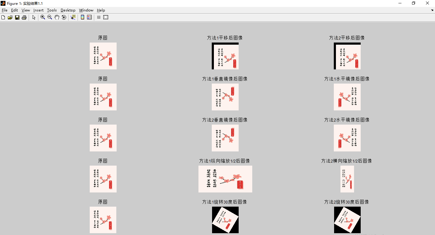
1.First part Experiments: Translation, Vertical Mirror Transformation, Horizontal Mirror Transformation, Scaling and Rotation
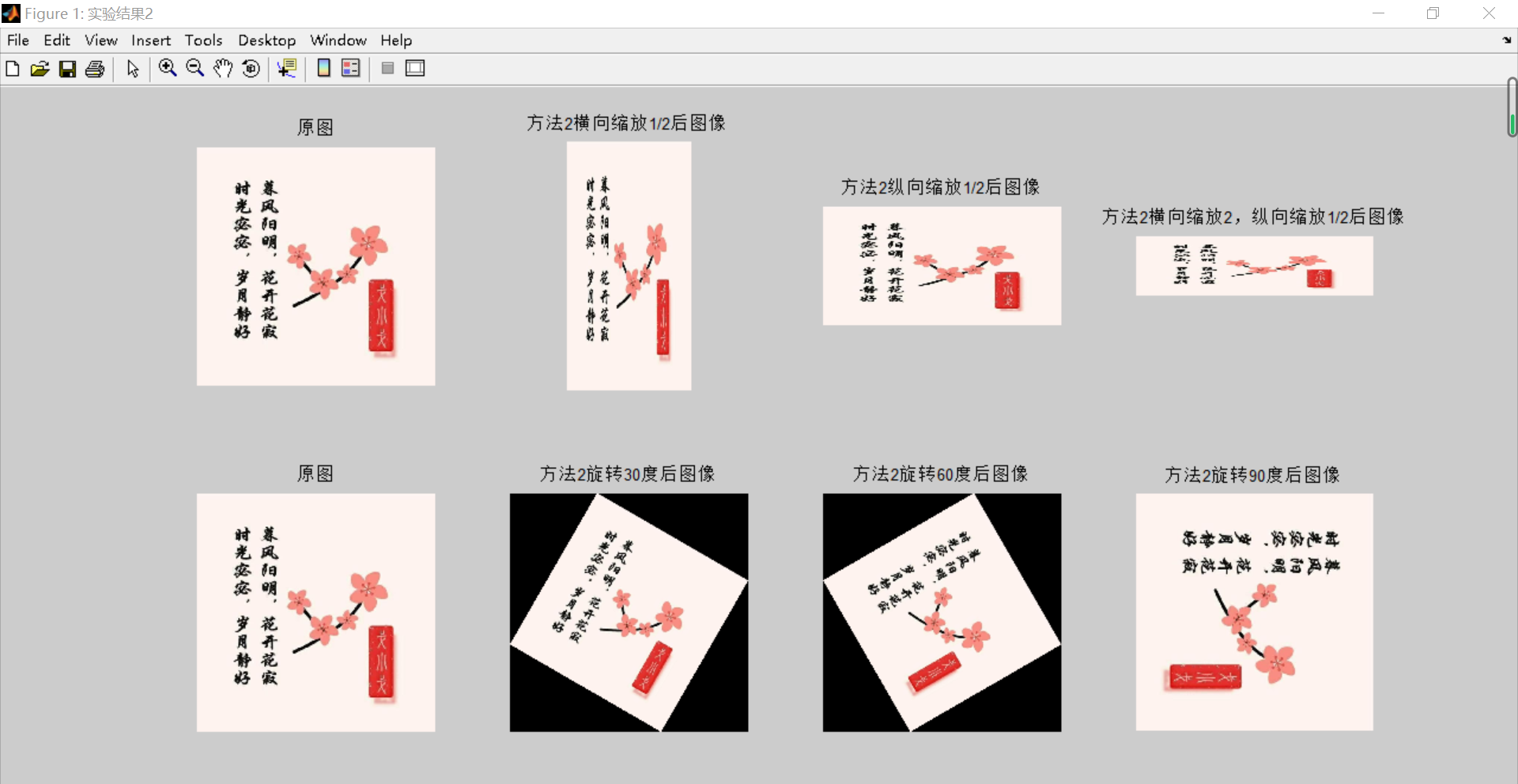
2. Second part: Experimental results: Changing image scaling ratio and rotation angle
3. The third part of the experiment results: the effect is not obvious in smaller pictures, but obvious after zooming in.

The code is as follows:
%1.1
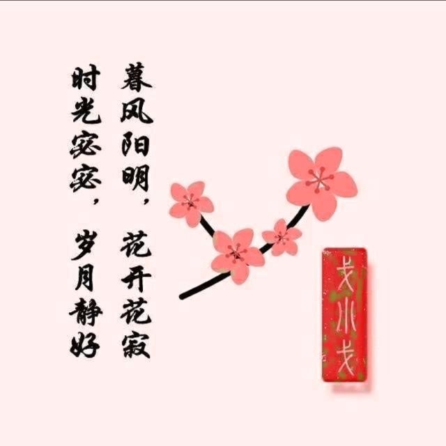
pic=imread('pic.png'); %Read in pictures'pic.png'
figure('name','Experimentation 1.1');
num=5;% Definition num Line Picture
subplot(num,3,1);
imshow(pic);
title('Original Map');
subplot(num,3,4);
imshow(pic);
title('Original Map');
subplot(num,3,7);
imshow(pic);
title('Original Map');
subplot(num,3,10);
imshow(pic);
title('Original Map');
subplot(num,3,13);
imshow(pic);
title('Original Map');
% The first method shifts by adding or subtracting two-dimensional matrices
[R, C, V] = size(pic); % Get Image Size
res = zeros(R, C, V); % Construct the result matrix. Each pixel point is initialized to 0 (black) by default
delX = 50; % Translation X
delY = 50; % Translation Y
tras = [1 0 delX; 0 1 delY; 0 0 1]; % Translation Matrix
r = zeros([R,C]);
g = zeros([R,C]);
b = zeros([R,C]);
temp1 = pic(:, :, 1);
temp2 = pic(:, :, 2);
temp3 = pic(:, :, 3);
for i = 1 : R
for j = 1 : C
x = i+delX;
y = j+delY;
% Transformed position judgement is out of bounds
if (x <= R) & (y <= C) & (x >= 1) & (y >= 1)
r(x,y) = temp1(i,j);
g(x,y) = temp2(i,j);
b(x,y) = temp3(i,j);
end
end
end;
res(:, :, 1) = r;
res(:, :, 2) = g;
res(:, :, 3) = b;
subplot(num,3,2);
imshow(uint8(res)); % Display Image
title('Method 1 Post-panning image');
% The second method uses a spatial transformation matrix translation
delX = 50; % Translation X
delY = 50; % Translation Y
xform=maketform('affine', [1 0 0; 0 1 0; delX delY 1]);%Implement image panning
res=imtransform(pic,xform,'XData',[1 size(pic,2)],'YData',[1 size(pic,1)]);%Perform image translation
subplot(num,3,3);
imshow(res); % Display Image
title('Method 2 Post-translational Image');
%1.2
% The first method uses a two-dimensional matrix to add and subtract images
for i = 1 : R
for j = 1 : C
% mirror vertically
r(R-i+1,j) = temp1(i,j);
g(R-i+1,j) = temp2(i,j);
b(R-i+1,j) = temp3(i,j);
end
end;
res(:, :, 1) = r;
res(:, :, 2) = g;
res(:, :, 3) = b;
subplot(num,3,5);
imshow(uint8(res)); % Display Image
title('Method 1 Image after vertical mirroring');
for i = 1 : R
for j = 1 : C
% Left and right mirror
r(i,C-j+1) = temp1(i,j);
g(i,C-j+1) = temp2(i,j);
b(i,C-j+1) = temp3(i,j);
end
end;
res(:, :, 1) = r;
res(:, :, 2) = g;
res(:, :, 3) = b;
subplot(num,3,6);
imshow(uint8(res)); % Display Image
title('Method 1 Image after Horizontal Mirroring');
% The second method mirrors the matrix by spatial transformation
%Vertical Mirror Transform
tform2 = maketform('affine', [1 0 0; 0 -1 0; 0 C 1]);
RES=imtransform(pic, tform2, 'nearest');
subplot(num,3,8);
imshow(RES); % Display Image
title('Method 2 Image after Vertical Mirroring');
%Horizontal Mirror Transform
tform = maketform('affine',[-1 0 0;0 1 0; R 0 1]);
RES=imtransform(pic, tform, 'nearest'); %Applying a two-dimensional spatial transformation to an image
subplot(num,3,9);
imshow(RES); % Display Image
title('Method 2 Image after Horizontal Mirroring');
%1.3
% The first method scales by adding or subtracting two-dimensional matrices
delX=1 %Scale Horizontally
delY=0.5 %Vertical Scale
res = zeros(R*delY, C*delX, V); % Construct the result matrix. Each pixel point is initialized to 0 (black) by default
r = zeros([R*delY, C*delX]);
g = zeros([R*delY, C*delX]);
b = zeros([R*delY, C*delX]);
for i = 1 : R*delY
for j = 1 : C*delX
x = floor(i / delY);
y = floor(j / delX);
u = (i / delY) - x;
v = (j / delX) - y;
if (x <= R) && (y <= C) && (x >= 1) && (y >= 1)
r(i,j) = temp1(floor(x), floor(y)) * (1-u) * (1-v) + temp1(floor(x), ceil(y)) * (1-u) * v + temp1(ceil(x), floor(y)) * u * (1-v) + temp1(ceil(x), ceil(y)) * u * v;
g(i,j) = temp2(floor(x), floor(y)) * (1-u) * (1-v) + temp2(floor(x), ceil(y)) * (1-u) * v + temp2(ceil(x), floor(y)) * u * (1-v) + temp2(ceil(x), ceil(y)) * u * v;
b(i,j) = temp3(floor(x), floor(y)) * (1-u) * (1-v) + temp3(floor(x), ceil(y)) * (1-u) * v + temp3(ceil(x), floor(y)) * u * (1-v) + temp3(ceil(x), ceil(y)) * u * v;
end
end
end;
res(:, :, 1) = r;
res(:, :, 2) = g;
res(:, :, 3) = b;
subplot(num,3,11);
imshow(uint8(res)); % Display Image
title('Method 1 Scale Longitudinally 1/2 Post image');
% The second method scales by a spatial transformation matrix
xform = maketform('affine', [0.5 0 0;0 1 0;0 0 1]);%[Horizontal zoom 0;0 Vertical zoom ratio 0;0 0 1]
RES=imtransform(pic, xform);
subplot(num,3,12);
imshow(RES); % Display Image
title('Method 2 Scale Horizontally 1/2 Post image');
%1.4
% The first method rotates by adding or subtracting two-dimensional matrices
angle=30;
theta=(angle / 180) * pi;
rotation_matrix=[cos(theta) -sin(theta) 0; sin(theta) cos(theta) 0; 0 0 1];
up_left=[1 1 1]*rotation_matrix;
up_right=[1 C 1]*rotation_matrix;
down_left=[R 1 1]*rotation_matrix;
down_right=[R C 1]*rotation_matrix;
height=round(max([abs(up_left(1)-down_right(1))+0.5 abs(up_right(1)-down_left(1))+0.5])); %Height of the transformed image
width=round(max([abs(up_left(2)-down_right(2))+0.5 abs(up_right(2)-down_left(2))+0.5])); %Width of transformed image
res = zeros([height,width,V]);
r = zeros([height,width]);
g = zeros([height,width]);
b = zeros([height,width]);
delta_y=abs(min([up_left(1) up_right(1) down_left(1) down_right(1)]));
delta_x=abs(min([up_left(2) up_right(2) down_left(2) down_right(2)]));
for i=1-delta_y:height-delta_y
for j=1-delta_x:width-delta_x
point = [i j 1]/rotation_matrix;
m = point(1);
n = point(2);
u=m-floor(m);
v=n-floor(n);
if (m <= R) && (n <= C) && (m >= 1) && (n >= 1)
r(i+delta_y,j+delta_x) = temp1(floor(m), floor(n)) * (1-u) * (1-v) + temp1(floor(m), ceil(n)) * (1-u) * v + temp1(ceil(m), floor(n)) * u * (1-v) + temp1(ceil(m), ceil(n)) * u * v;
g(i+delta_y,j+delta_x) = temp2(floor(m), floor(n)) * (1-u) * (1-v) + temp2(floor(m), ceil(n)) * (1-u) * v + temp2(ceil(m), floor(n)) * u * (1-v) + temp2(ceil(m), ceil(n)) * u * v;
b(i+delta_y,j+delta_x) = temp3(floor(m), floor(n)) * (1-u) * (1-v) + temp3(floor(m), ceil(n)) * (1-u) * v + temp3(ceil(m), floor(n)) * u * (1-v) + temp3(ceil(m), ceil(n)) * u * v;
end
end
end
res(:, :, 1) = r;
res(:, :, 2) = g;
res(:, :, 3) = b;
subplot(num,3,14);
imshow(uint8(res)); % Display Image
title('Method 1 Rotate the image 30 degrees');
% The second method rotates through a spatial transformation matrix
xform = maketform('affine',[cosd(-angle) -sind(-angle) 0; sind(-angle) cosd(-angle) 0; 0 0 1]);%Create Rotation Parameter Structures
RES=imtransform(pic, xform);
subplot(num,3,15);
imshow(RES); % Display Image
title('Method 2 Rotates the image 30 degrees');
Part 2 Code: Change the scale and rotation of the image
%2
pic=imread('pic.png'); %Read in pictures'pic.png'
figure('name','Experimentation 2');
num=2;% Definition num Line Picture
subplot(num,4,1);
imshow(pic);
title('Original Map');
subplot(num,4,5);
imshow(pic);
title('Original Map');
% The second method scales by a spatial transformation matrix
xform = maketform('affine', [0.5 0 0;0 1 0;0 0 1]);%[Horizontal zoom 0;0 Vertical zoom ratio 0;0 0 1]
RES=imtransform(pic, xform);
subplot(num,4,2);
imshow(RES); % Display Image
title('Method 2 Scale Horizontally 1/2 Post image');
xform = maketform('affine', [1 0 0;0 0.5 0;0 0 1]);%[Horizontal zoom 0;0 Vertical zoom ratio 0;0 0 1]
RES=imtransform(pic, xform);
subplot(num,4,3);
imshow(RES); % Display Image
title('Method 2 Vertical zoom 1/2 Post image');
xform = maketform('affine', [2 0 0;0 0.5 0;0 0 1]);%[Horizontal zoom 0;0 Vertical zoom ratio 0;0 0 1]
RES=imtransform(pic, xform);
subplot(num,4,4);
imshow(RES); % Display Image
title('Method 2 Scale 2 horizontally and 1 vertically/2 Post image');
% The second method rotates through a spatial transformation matrix
angle=30;
xform = maketform('affine',[cosd(-angle) -sind(-angle) 0; sind(-angle) cosd(-angle) 0; 0 0 1]);%Create Rotation Parameter Structures
RES=imtransform(pic, xform);
subplot(num,4,6);
imshow(RES); % Display Image
title('Method 2 Rotates the image 30 degrees');
angle=60;
xform = maketform('affine',[cosd(-angle) -sind(-angle) 0; sind(-angle) cosd(-angle) 0; 0 0 1]);%Create Rotation Parameter Structures
RES=imtransform(pic, xform);
subplot(num,4,7);
imshow(RES); % Display Image
title('Method 2 Rotate the image 60 degrees');
angle=90;
xform = maketform('affine',[cosd(-angle) -sind(-angle) 0; sind(-angle) cosd(-angle) 0; 0 0 1]);%Create Rotation Parameter Structures
RES=imtransform(pic, xform);
subplot(num,4,8);
imshow(RES); % Display Image
title('Method 2 Rotates the image 90 degrees');
Part Three Code:
%3
pic=imread('pic.png'); %Read in pictures'pic.png'
figure('name','Experimental result 3');
number=4;% Definition number Line Picture
subplot(number,3,1);
imshow(pic);
title('RGB Original Map');
subplot(number,3,4);
imshow(pic);
title('HSI Original Map');
subplot(number,3,7);
imshow(pic);
title('HSI Original Map');
subplot(number,3,10);
imshow(pic);
title('HSI Original Map');
% RGB Fuzzy Processing
r=pic(:,:,1);
g=pic(:,:,2);
b=pic(:,:,3);
m=fspecial('average');
r_filtered=imfilter(r,m);
g_filtered=imfilter(g,m);
b_filtered=imfilter(b,m);
pic_filtered=cat(3,r_filtered,g_filtered,b_filtered);
subplot(number,3,2);
imshow(pic_filtered);
title('RGB Fuzzy Processing');
% RGB Crisp Enhancement
lapMatrix=[1 1 1;1 -8 1;1 1 1];
i_tmp=imfilter(pic_filtered,lapMatrix,'replicate');
i_sharped=imsubtract(pic,i_tmp);
subplot(number,3,3);
imshow(i_sharped);
title('RGB Crisp Enhancement');
%HSI
% Extracting image components
pic = im2double(pic);
r = pic(:, :, 1);
g = pic(:, :, 2);
b = pic(:, :, 3);
% Perform the conversion equation
num = 0.5*((r - g) + (r - b));
den = sqrt((r - g).^2 + (r - b).*(g - b));
theta = acos(num./(den + eps)); %Prevent division by 0
H = theta;
H(b > g) = 2*pi - H(b > g);
H = H/(2*pi);
num = min(min(r, g), b);
den = r + g + b;
den(den == 0) = eps; %Prevent division by 0
S = 1 - 3.* num./den;
H(S == 0) = 0;
I = (r + g + b)/3;
% Combine three components into one HSI image
hsi = cat(3, H, S, I);
% HSI,Yes H Component image blurring
m = fspecial('average', [8, 8]);
H = imfilter(H, m);
% Implement the conversion equations.
R = zeros(size(hsi, 1), size(hsi, 2));
G = zeros(size(hsi, 1), size(hsi, 2));
B = zeros(size(hsi, 1), size(hsi, 2));
% RG sector (0 <= H < 2*pi/3).
idx = find( (0 <= H) & (H < 2*pi/3));
B(idx) = I(idx) .* (1 - S(idx));
R(idx) = I(idx) .* (1 + S(idx) .* cos(H(idx)) ./ cos(pi/3 - H(idx)));
G(idx) = 3*I(idx) - (R(idx) + B(idx));
% BG sector (2*pi/3 <= H < 4*pi/3).
idx = find( (2*pi/3 <= H) & (H < 4*pi/3) );
R(idx) = I(idx) .* (1 - S(idx));
G(idx) = I(idx) .* (1 + S(idx) .* cos(H(idx) - 2*pi/3) ./ cos(pi - H(idx)));
B(idx) = 3*I(idx) - (R(idx) + G(idx));
% BR sector.
idx = find( (4*pi/3 <= H) & (H <= 2*pi));
G(idx) = I(idx) .* (1 - S(idx));
B(idx) = I(idx) .* (1 + S(idx) .* cos(H(idx) - 4*pi/3) ./cos(5*pi/3 - H(idx)));
R(idx) = 3*I(idx) - (G(idx) + B(idx));
rgb = cat(3, R, G, B);
rgb = max(min(rgb, 1), 0);
subplot(number,3,5);
imshow(rgb);
title('H After blurring component');
%sharpening
lapMatrix=[1 1 1;1 -8 1;1 1 1];
i_tmp=imfilter(H,lapMatrix,'replicate');
H_sharped=imsubtract(H,i_tmp);
hsi = cat(3,H_sharped,S,I);
% Implement the conversion equations.
R = zeros(size(hsi, 1), size(hsi, 2));
G = zeros(size(hsi, 1), size(hsi, 2));
B = zeros(size(hsi, 1), size(hsi, 2));
% RG sector (0 <= H < 2*pi/3).
idx = find( (0 <= H) & (H < 2*pi/3));
B(idx) = I(idx) .* (1 - S(idx));
R(idx) = I(idx) .* (1 + S(idx) .* cos(H(idx)) ./ cos(pi/3 - H(idx)));
G(idx) = 3*I(idx) - (R(idx) + B(idx));
% BG sector (2*pi/3 <= H < 4*pi/3).
idx = find( (2*pi/3 <= H) & (H < 4*pi/3) );
R(idx) = I(idx) .* (1 - S(idx));
G(idx) = I(idx) .* (1 + S(idx) .* cos(H(idx) - 2*pi/3) ./ cos(pi - H(idx)));
B(idx) = 3*I(idx) - (R(idx) + G(idx));
% BR sector.
idx = find( (4*pi/3 <= H) & (H <= 2*pi));
G(idx) = I(idx) .* (1 - S(idx));
B(idx) = I(idx) .* (1 + S(idx) .* cos(H(idx) - 4*pi/3) ./cos(5*pi/3 - H(idx)));
R(idx) = 3*I(idx) - (G(idx) + B(idx));
rgb = cat(3, R, G, B);
rgb = max(min(rgb, 1), 0);
subplot(number,3,6);
imshow(rgb);
title('H After component sharpening');
%S Component blurring
m=fspecial('average',[8,8]);
s_filtered=imfilter(S,m);
hsi = cat(3,H,s_filtered,I);
% Implement the conversion equations.
R = zeros(size(hsi, 1), size(hsi, 2));
G = zeros(size(hsi, 1), size(hsi, 2));
B = zeros(size(hsi, 1), size(hsi, 2));
% RG sector (0 <= H < 2*pi/3).
idx = find( (0 <= H) & (H < 2*pi/3));
B(idx) = I(idx) .* (1 - S(idx));
R(idx) = I(idx) .* (1 + S(idx) .* cos(H(idx)) ./ cos(pi/3 - H(idx)));
G(idx) = 3*I(idx) - (R(idx) + B(idx));
% BG sector (2*pi/3 <= H < 4*pi/3).
idx = find( (2*pi/3 <= H) & (H < 4*pi/3) );
R(idx) = I(idx) .* (1 - S(idx));
G(idx) = I(idx) .* (1 + S(idx) .* cos(H(idx) - 2*pi/3) ./ cos(pi - H(idx)));
B(idx) = 3*I(idx) - (R(idx) + G(idx));
% BR sector.
idx = find( (4*pi/3 <= H) & (H <= 2*pi));
G(idx) = I(idx) .* (1 - S(idx));
B(idx) = I(idx) .* (1 + S(idx) .* cos(H(idx) - 4*pi/3) ./cos(5*pi/3 - H(idx)));
R(idx) = 3*I(idx) - (G(idx) + B(idx));
rgb = cat(3, R, G, B);
rgb = max(min(rgb, 1), 0);
subplot(number,3,8);
imshow(rgb);
title('S After blurring component');
%S Component sharpening
lapMatrix=[1 1 1;1 -8 1;1 1 1];
i_tmp=imfilter(S,lapMatrix,'replicate');
s_sharped=imsubtract(S,i_tmp);
hsi = cat(3,H,s_sharped,I);
% Implement the conversion equations.
R = zeros(size(hsi, 1), size(hsi, 2));
G = zeros(size(hsi, 1), size(hsi, 2));
B = zeros(size(hsi, 1), size(hsi, 2));
% RG sector (0 <= H < 2*pi/3).
idx = find( (0 <= H) & (H < 2*pi/3));
B(idx) = I(idx) .* (1 - S(idx));
R(idx) = I(idx) .* (1 + S(idx) .* cos(H(idx)) ./ cos(pi/3 - H(idx)));
G(idx) = 3*I(idx) - (R(idx) + B(idx));
% BG sector (2*pi/3 <= H < 4*pi/3).
idx = find( (2*pi/3 <= H) & (H < 4*pi/3) );
R(idx) = I(idx) .* (1 - S(idx));
G(idx) = I(idx) .* (1 + S(idx) .* cos(H(idx) - 2*pi/3) ./ cos(pi - H(idx)));
B(idx) = 3*I(idx) - (R(idx) + G(idx));
% BR sector.
idx = find( (4*pi/3 <= H) & (H <= 2*pi));
G(idx) = I(idx) .* (1 - S(idx));
B(idx) = I(idx) .* (1 + S(idx) .* cos(H(idx) - 4*pi/3) ./cos(5*pi/3 - H(idx)));
R(idx) = 3*I(idx) - (G(idx) + B(idx));
rgb = cat(3, R, G, B);
rgb = max(min(rgb, 1), 0);
subplot(number,3,9);
imshow(rgb);
title('S After component sharpening');
%I Component blurring
m=fspecial('average',[8,8]);
i_filtered=imfilter(I,m);
hsi = cat(3,H,S,i_filtered);
% Implement the conversion equations.
R = zeros(size(hsi, 1), size(hsi, 2));
G = zeros(size(hsi, 1), size(hsi, 2));
B = zeros(size(hsi, 1), size(hsi, 2));
% RG sector (0 <= H < 2*pi/3).
idx = find( (0 <= H) & (H < 2*pi/3));
B(idx) = I(idx) .* (1 - S(idx));
R(idx) = I(idx) .* (1 + S(idx) .* cos(H(idx)) ./ cos(pi/3 - H(idx)));
G(idx) = 3*I(idx) - (R(idx) + B(idx));
% BG sector (2*pi/3 <= H < 4*pi/3).
idx = find( (2*pi/3 <= H) & (H < 4*pi/3) );
R(idx) = I(idx) .* (1 - S(idx));
G(idx) = I(idx) .* (1 + S(idx) .* cos(H(idx) - 2*pi/3) ./ cos(pi - H(idx)));
B(idx) = 3*I(idx) - (R(idx) + G(idx));
% BR sector.
idx = find( (4*pi/3 <= H) & (H <= 2*pi));
G(idx) = I(idx) .* (1 - S(idx));
B(idx) = I(idx) .* (1 + S(idx) .* cos(H(idx) - 4*pi/3) ./cos(5*pi/3 - H(idx)));
R(idx) = 3*I(idx) - (G(idx) + B(idx));
rgb = cat(3, R, G, B);
rgb = max(min(rgb, 1), 0);
subplot(number,3,11);
imshow(rgb);
title('I After blurring component');
%I Component sharpening
lapMatrix=[1 1 1;1 -8 1;1 1 1];
i_tmp=imfilter(I,lapMatrix,'replicate');
i_sharped=imsubtract(I,i_tmp);
hsi = cat(3,H,S,i_sharped);
% Implement the conversion equations.
R = zeros(size(hsi, 1), size(hsi, 2));
G = zeros(size(hsi, 1), size(hsi, 2));
B = zeros(size(hsi, 1), size(hsi, 2));
% RG sector (0 <= H < 2*pi/3).
idx = find( (0 <= H) & (H < 2*pi/3));
B(idx) = I(idx) .* (1 - S(idx));
R(idx) = I(idx) .* (1 + S(idx) .* cos(H(idx)) ./ cos(pi/3 - H(idx)));
G(idx) = 3*I(idx) - (R(idx) + B(idx));
% BG sector (2*pi/3 <= H < 4*pi/3).
idx = find( (2*pi/3 <= H) & (H < 4*pi/3) );
R(idx) = I(idx) .* (1 - S(idx));
G(idx) = I(idx) .* (1 + S(idx) .* cos(H(idx) - 2*pi/3) ./ cos(pi - H(idx)));
B(idx) = 3*I(idx) - (R(idx) + G(idx));
% BR sector.
idx = find( (4*pi/3 <= H) & (H <= 2*pi));
G(idx) = I(idx) .* (1 - S(idx));
B(idx) = I(idx) .* (1 + S(idx) .* cos(H(idx) - 4*pi/3) ./cos(5*pi/3 - H(idx)));
R(idx) = 3*I(idx) - (G(idx) + B(idx));
rgb = cat(3, R, G, B);
rgb = max(min(rgb, 1), 0);
subplot(number,3,12);
imshow(rgb);
title('I After component sharpening');
imwrite(rgb, 'I After component sharpening.jpg');