1. Topic 1

1. The zero pole gain models of known systems are:

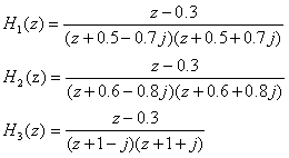
The zero pole distribution diagram and impulse response of these systems are obtained, and the causal stability of the system is judged. (answer with matlab)

Since the zero pole gain model given in the topic needs to be converted into the system function transfer model, and then zplane is used for zero pole analysis. The results are shown as follows:

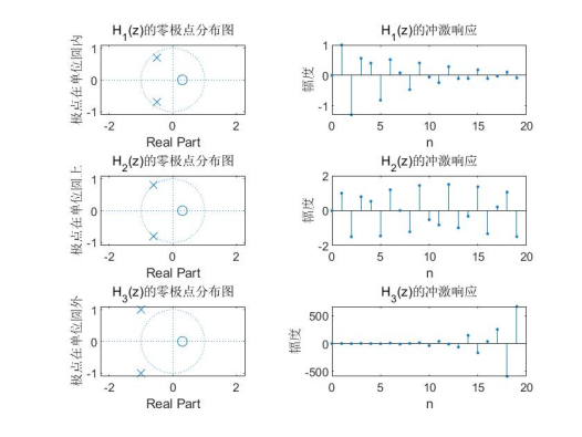
Judging from the above zero pole diagram:
① For H1(z), all its poles are located in the unit circle, so the system is causal stable;
② For H2(z), the impulse response is not 0 only when n ≥ 0, which is a causal system; All the poles are located on the unit circle, and the impulse response curve of the system is equal amplitude oscillation, which is not satisfied with absolute additive and unstable, so it is not causal stable system;
③ For H3(z), its impulse response is not 0 only when n ≥ 0, which is a causal system; All poles are located outside the unit circle, and the impulse response of the system diverges with the increase of frequency, which is not absolutely summable and unstable, so it is not a causal stable system.

z1=[0.3]';p1=[-0.5+0.7*1j,-0.5-0.7*1j]';k1=1;%zpk model parameter 
[b1,a1]=zp2tf(z1,p1,k1);            %Transformed into system transfer function model
subplot(3,2,1),zplane(b1,a1);
ylabel('The pole is in the unit circle');title('H_1(z)Zero pole distribution diagram of');
subplot(3,2,2);
[y1,x1]=impz(b1,a1,20);stem(x1,y1,'.');
xlabel('n');ylabel('range');title('H_1(z)Impulse response of')

z2=[0.3]';p2=[-0.6+0.8*1j,-0.6-0.8*1j]';k2=1;%zpk model parameter 
[b2,a2]=zp2tf(z2,p2,k2);            %Transformed into system transfer function model
subplot(3,2,3),zplane(b2,a2);
ylabel('The pole is on the unit circle');title('H_2(z)Zero pole distribution diagram of');
subplot(3,2,4);
[y2,x2]=impz(b2,a2,20);stem(x2,y2,'.');
xlabel('n');ylabel('range');title('H_2(z)Impulse response of')

z3=[0.3]';p3=[-1+1j,-1-1j];k3=1;%zpk model parameter 
[b3,a3]=zp2tf(z3,p3,k3);            %Transformed into system transfer function model
subplot(3,2,5),zplane(b3,a3);
ylabel('The pole is outside the unit circle');title('H_3(z)Zero pole distribution diagram of');
subplot(3,2,6);
[y3,x3]=impz(b3,a3,20);stem(x3,y3,'.');
xlabel('n');ylabel('range');title('H_3(z)Impulse response of')

2. Topic 2

2. Transfer function of known discrete-time system:

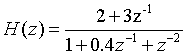
The relative amplitude frequency response and phase frequency response curve of the system in the frequency range of 0 - π are obtained. (answer with python)

Use SciPy The frequency response can be calculated by the freqz function in signal, and the results are as follows:

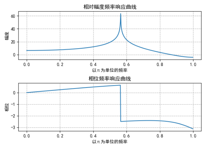
Where the unit of relative amplitude frequency response is dB instead of V.

import matplotlib.pyplot as plt
import numpy as np
from scipy import signal

plt.rcParams['font.sans-serif']=['SimHei'] #Used to display Chinese labels normally
plt.rcParams['axes.unicode_minus']=False #Used to display negative signs normally

a = np.array([1,0.4,1])#denominator
b = np.array([2,3,0])
w,h = signal.freqz(b,a)#Calculate frequency response
w=w/np.pi   

plt.subplot(2,1,1)
plt.plot(w,20*np.log10(abs(h)))#Draw the relative amplitude frequency response curve
plt.title('Relative amplitude frequency response curve')
plt.xlabel('withπFrequency in')
plt.ylabel('range')
plt.grid(ls='--')#Generate gridlines

plt.subplot(2,1,2)
plt.plot(w,np.angle(h))#Draw the relative amplitude frequency response curve
plt.title('Phase frequency response curve')
plt.xlabel('withπFrequency in')
plt.ylabel('phase')
plt.grid(ls='--')#Generate gridlines
plt.tight_layout()
plt.show()

3. Topic 3

It is known that the zero pole gain model of discrete-time system is:

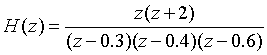
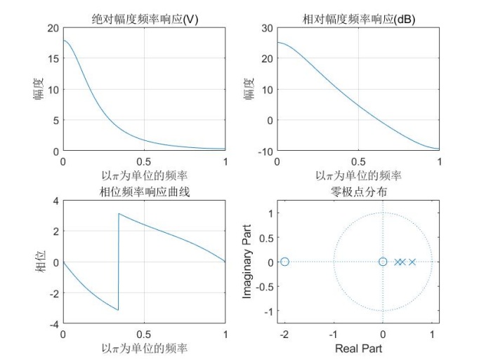
The absolute amplitude frequency response, relative amplitude frequency response, phase frequency response curve and zero pole distribution diagram of the system in the frequency range of 0 - π are obtained. (answer with matlab)

The zero pole gain model given in the topic should be transformed into the system transfer function model before using freqz to solve the frequency response. The absolute frequency response is the absolute value of amplitude, while the relative frequency response is the absolute frequency response, which is converted into the form in dB. The phase frequency response can be solved by angle function, and the zero pole distribution diagram can be solved by zplane function. The results obtained are as follows:

z=[0,-2]';p=[0.3,0.4,0.6]';k=1;%zpk model parameter 
[b,a]=zp2tf(z,p,k);%Transformed into system transfer function model
n=(0:500)*pi/500;%stay pi 501 sampling points are taken within the range of
[h,w]=freqz(b,a,n);%Find the frequency response of the system
subplot(2,2,1),plot(w/pi,abs(h));grid;
xlabel('with\pi Frequency in');ylabel('range');
title('Absolute amplitude frequency response(V)');

dB=20*log10(abs(h));    %Find the relative amplitude frequency response curve of the system
subplot(2,2,2),plot(w/pi,dB);grid;
xlabel('with\pi Frequency in');ylabel('range');
title('Relative amplitude frequency response(dB)');

subplot(2,2,3),plot(w/pi,angle(h));grid;%Phase frequency response diagram
xlabel('with\pi Frequency in');ylabel('phase');
title('Phase frequency response curve');

subplot(2,2,4),zplane(b,a);%Zero pole distribution diagram
title('Zero pole distribution');

4. Topic 4

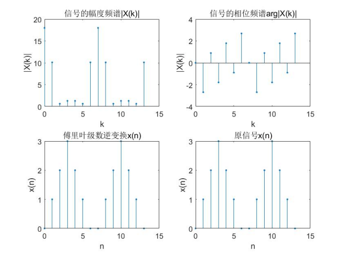
4. It is known that the principal value of a signal sequence is x(n)=[0,1,2,3,2,1,0], and the signal sequence waveform of 2 cycles is displayed. requirement:
① The amplitude spectrum and phase spectrum of the signal are obtained by Fourier series transform and represented graphically.
② The graph of Fourier series inverse transform is obtained and compared with the original signal graph. (answer with matlab)

The cumulative summation of Fourier series can be realized by matrix multiplication. Since the periodic sequence is twice the original principal value sequence, the amplitude of the signal will be expanded by 22 times after direct inverse transformation. Therefore, the amplitude of the signal after inverse transformation should be divided by 22. The results are as follows:

x=[0,1,2,3,2,1,0];
xn=[x,x];%Displays a signal sequence of two cycles
N=7;
n=0:2*N-1;
k=0:2*N-1;
Xk=xn*exp(-1j*2*pi/N).^(n'*k);%Discrete Fourier series transform
x_idfs=(Xk*exp(1j*2*pi/N).^(n'*k))/(2*2*N);%Inverse discrete Fourier series transform

subplot(2,2,1),stem(k,abs(Xk),'.');
xlabel('k');ylabel('|X(k)|');
title('Amplitude spectrum of signal|X(k)|');

subplot(2,2,2),stem(k,angle(Xk),'.');
xlabel('k');ylabel('|X(k)|');
title('Phase spectrum of signal arg|X(k)|');

subplot(2,2,3),stem(n,real(x_idfs),'.');
xlabel('n');ylabel('x(n)');
title('Inverse Fourier series transform x(n)');

subplot(2,2,4),stem(n,xn,'.');
xlabel('n');ylabel('x(n)');
title('Original signal x(n)');

5. Topic 5

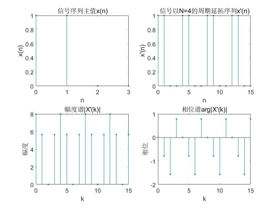
It is known that the principal value of a signal sequence is x(n)=R2(n),. requirement:
① Show x(n) andGraphics for.
② Fourier series transform is used to calculate and displayImage. (answer with matlab)

The periodic sequence is plotted in 4 cycles, and the results are as follows:

N=4;%Periodic continuation with 4 as cycle
xn=[1,1,0,0];
n=0:N-1;
k=0:N-1;
n1=0:4*N-1;%Drawing by extending four periods
k1=0:4*N-1;
x1=[xn,xn,xn,xn];
Xk=x1*exp(-1j*2*pi/N).^(n1'*k1);%Discrete Fourier series transform

subplot(2,2,1),stem(n,xn,'.');
title('Signal sequence principal value x(n)');
xlabel('n'),ylabel('x(n)');

subplot(2,2,2),stem(n1,x1,'.');
title('Signal to N=4 Periodic continuation sequence of x''(n)');
xlabel('n'),ylabel('x''(n)');

subplot(2,2,3),stem(k1,abs(Xk),'.');
title('Amplitude spectrum|X''(k)|');
xlabel('k'),ylabel('range');

subplot(2,2,4),stem(k1,angle(Xk),'.');
title('Phase spectrum arg|X''(k)|');
xlabel('k'),ylabel('phase');

6. Topic 6

Given the finite length sequence x(n)=[7,6,5,4,3,2], find the DFT and IDFT of x(n).
Requirements: ① draw the graphics of | X(k) | and arg[|X(k) |] corresponding to Fourier transform;
② Draw the original signal and compare it with the inverse Fourier transform IDFT[X(k)]. (answer with matlab)

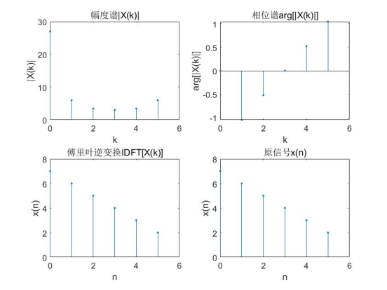
It can be seen from the above figure that the signal obtained by inverse Fourier transform is the same as the original signal x(n), and the result is correct.

xn=[7,6,5,4,3,2];%Signal sequence
N=length(xn);
n=0:N-1;k=0:N-1;
Xk=xn*exp(-1j*2*pi/N).^(n'*k);%Discrete Fourier transform
x=(Xk*exp(1j*2*pi/N).^(n'*k))/N;%Inverse discrete Fourier transform

subplot(2,2,1);stem(k,abs(Xk),'.');
xlabel('k');ylabel('|X(k)|');
title('Amplitude spectrum|X(k)|');

subplot(2,2,2);stem(k,angle(Xk),'.');
xlabel('k');ylabel('arg[|X(k)|]');
title('Phase spectrum arg[|X(k)|]');

subplot(2,2,3);stem(n,real(x),'.');
xlabel('n');ylabel('x(n)');
title('Inverse Fourier transform IDFT[X(k)]');

subplot(2,2,4);stem(n,xn,'.');
xlabel('n');ylabel('x(n)');
title('Original signal x(n)');

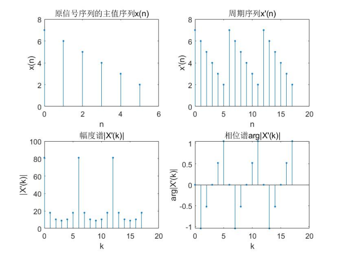
7. Topic VII

Given the principal value x(n)=[7,6,5,4,3,2] of the periodic sequence, find the DFS and IDFS when the number of x(n) periodic repetitions is 3. Requirements: ① draw the graph of the principal value and periodic sequence of the original signal sequence;
② Draw the sequence corresponding to Fourier transformGraphics for. (answer with matlab)

xn=[7,6,5,4,3,2];%Principal value sequence of periodic sequence
N=length(xn);
n=0:N-1;
xn1=[xn,xn,xn];%x(n)The cycle is repeated three times
n1=0:3*N-1;
k1=0:3*N-1;
Xk=xn1*exp(-1j*2*pi/N).^(n1'*k1);
x=(Xk*exp(1j*2*pi/N).^(n1'*k1))/(3*3*N);

subplot(2,2,1),stem(n,xn,'.');
xlabel('n'),ylabel('x(n)');
title('Principal value sequence of original signal sequence x(n)');

subplot(2,2,2),stem(n1,xn1,'.');
xlabel('n'),ylabel('x''(n)');
title('Periodic sequence x''(n)');

subplot(2,2,3),stem(k1,abs(Xk),'.');
xlabel('k'),ylabel('|X''(k)|');
title('Amplitude spectrum|X''(k)|');

subplot(2,2,4),stem(k1,angle(Xk),'.');
xlabel('k'),ylabel('arg|X''(k)|');
title('Phase spectrum arg|X''(k)|');