1. Topic 1

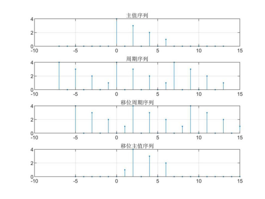
Given the finite length sequence x(n) = [4,0,3,0,2,0,1], find that x(n) shifts 2 bits to the right to become a new vector y(n), and draw the intermediate process of cyclic shift. (answer with matlab)

Firstly, the sequence of x(n) is established, and then the shift operation is carried out after periodic extension. Finally, the circularly shifted sequence can be obtained by taking the principal value sequence. The results are as follows:

%question 1
clear;
xn=[4,0,3,0,2,0,1];%establish xn sequence
Nx=length(xn);
nx=0:Nx-1;
nx1=-Nx:2*Nx-1;%Establish the scope of periodic continuation
x1=xn(mod(nx1,Nx)+1);%Establish periodic continuation sequence
ny1=nx1+2;y1=x1;%take x1 Shift 2 bits right to get y1
RN=(nx1>=0)&(nx1<Nx);%stay x1 Position vector of nx1 Upper setting main value window
RN1=(ny1>=0)&(ny1<Nx);%stay y1 Position vector of ny1 Upper setting main value window
subplot(4,1,1),stem(nx1,RN.*x1,'.');%Draw x1 Main value part of
axis([-10,15,0,4]);title('Principal value sequence');grid on
subplot(4,1,2),stem(nx1,x1,'.');%Draw x1
axis([-10,15,0,4]);title('Periodic sequence');grid on
subplot(4,1,3),stem(ny1,y1,'.');%Draw y1
axis([-10,15,0,4]);title('Shift period sequence');grid on
subplot(4,1,4),stem(ny1,RN1.*y1,'.');%Draw y1 Main value part of
axis([-10,15,0,4]);title('Shift principal value sequence');grid on

2. Topic 2

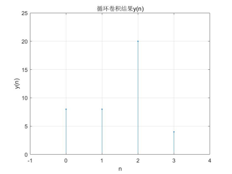
Two finite length sequences x1= [5,4,-3,-2], x2=[1,2,3,0] are known. The time-domain cyclic convolution y(n) is obtained by DFT and expressed graphically. (answer with matlab)

Calculate the DFT of two sequences x1 and x2 respectively, multiply them and then calculate the inverse transformation to obtain y(n), which is the result of time-domain cyclic convolution:

%question 2
clear;
xn1=[5,4,-3,-2];%establish x1(n)sequence
xn2=[1,2,3,0];%establish x2(n)Zulie
N=length(xn1);
n=0:N-1;k=0:N-1;
Xk1=xn1*(exp(-1j*2*pi/N)).^(n'*k);%from x1(n)of DFT seek X1(k)
Xk2=xn2*(exp(-1j*2*pi/N)).^(n'*k);%from x2(n)of DFT seek X2(k)
Yk=Xk1.*Xk2;%Y(k)=X1(k)X2(k)
yn=Yk*(exp(1j*2*pi/N)).^(n'*k)/N;%from Y(k)of IDFT seek y(n)
yn=abs(yn);%Modulus value, elimination DFT Small complex impact
stem(n,yn,'.');axis([-1,4,0,25])
title('Cyclic convolution result y(n)');
xlabel('n');ylabel('y(n)');grid on 

3. Topic 3

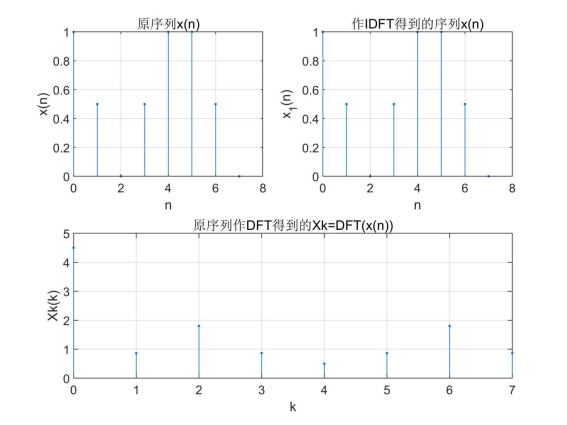
Known finite length sequence x(n) = [1,0.5,0,0.5,1,1,0.5,0], requirements:
① The DFT and IDFT graphs of the time-domain sequence are obtained by FFT algorithm;
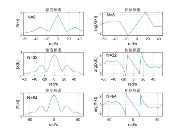
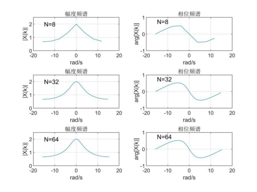
② Assuming that the sampling frequency F =20 Hz and the sequence length N is 8, 32 and 64 respectively, FFT is used to calculate its amplitude spectrum and phase spectrum. (answer with matlab)

The DFT of time-domain sequence is obtained by FFT and the time-domain sequence is obtained by IFFT. Through image comparison, it can be found that the time-domain sequence obtained by IFFT is the same as the original sequence, and the result is correct.

The spectrum of the sampled signal is obtained by fft function, and the amplitude spectrum and phase spectrum are obtained by abs and angle. The results are as follows:
It can be seen that the greater the value of N, the longer the sequence is retained, and the higher the accuracy of the spectrum curve.

%question 3
clear;
xn=[1,0.5,0,0.5,1,1,0.5,0];%establish x(n)sequence
N=length(xn);
n=0:N-1;k=0:N-1;
Xk=fft(xn,N);%do FFT
xn1=ifft(Xk,N);%do IFFT
subplot(2,2,1);stem(n,xn,'.');
title('Original sequence x(n)');grid on
xlabel('n');ylabel('x(n)');
subplot(2,1,2);stem(k,abs(Xk),'.');
title('Original sequence DFT Get Xk=DFT(x(n))');grid on
xlabel('k');ylabel('Xk(k)');
subplot(2,2,2);stem(n,xn1,'.');
title('do IDFT Obtained sequence x(n)');grid on
xlabel('n');ylabel('x_1(n)');


Fs=20;%sampling frequency  Fs=20Hz
N1=8;N2=32;N3=64;%Sequence length
D1=2*pi*Fs/N1;%Calculate analog frequency resolution
k1=floor(-(N1-1)/2:(N1-1)/2);%Frequency display range for[-π，π]
D2=2*pi*Fs/N2;%Calculate analog frequency resolution
k2=floor(-(N2-1)/2:(N2-1)/2);%Frequency display range for[-π，π]
D3=2*pi*Fs/N3;%Calculate analog frequency resolution
k3=floor(-(N3-1)/2:(N3-1)/2);%Frequency display range for[-π，π]
Xk1=fftshift(fft(xn,N1));%do FFT And shiftπ
Xk2=fftshift(fft(xn,N2));%do FFT And shiftπ
Xk3=fftshift(fft(xn,N3));%do FFT And shiftπ
figure;
subplot(3,2,1);plot(k1*D1,abs(Xk1))%Amplitude spectrum
title('Amplitude spectrum');xlabel('rad/s');ylabel('|X(k)|');
text(-55,4,'N=8');grid on
subplot(3,2,2);plot(k1*D1,angle(Xk1))%Phase spectrum
title('Phase spectrum');xlabel('rad/s');ylabel('arg[X(k)]');
text(-55,2,'N=8');grid on
subplot(3,2,3);plot(k2*D2,abs(Xk2))%Amplitude spectrum
title('Amplitude spectrum');xlabel('rad/s');ylabel('|X(k)|');
text(-55,4,'N=32');grid on
subplot(3,2,4);plot(k2*D2,angle(Xk2))%Phase spectrum
title('Phase spectrum');xlabel('rad/s');ylabel('arg[X(k)]');
text(-55,2,'N=32');grid on
subplot(3,2,5);plot(k3*D3,abs(Xk3))%Amplitude spectrum
title('Amplitude spectrum');xlabel('rad/s');ylabel('|X(k)|');
text(-55,4,'N=64');grid on
subplot(3,2,6);plot(k3*D3,angle(Xk3))%Phase spectrum
title('Phase spectrum');xlabel('rad/s');ylabel('arg[X(k)]');
text(-55,2,'N=64');grid on

4. Topic 4

An infinite sequence x(n)=0.5n(n ≥ 0) is known, and the sampling period TS = 0.2S. The sequence length n is required to be 8, 32 and 64 respectively, and its spectrum is calculated by FFT. (answer with matlab)

It can be seen from the image that the greater the value of N, the longer the sequence is retained, and the higher the accuracy of the spectrum curve.

%question 4
clear;
Ts=0.2;%The sampling period is T=0.2s
N1=[8,32,64];%Sequence length N
for r = 0:2
    N=N1(r+1);
    n=0:N-1;
    xn=0.5.^n;%establish x(n)
    D=2*pi/(N*Ts);
    k=floor(-(N-1)/2:(N-1)/2);
    X=fftshift(fft(xn,N));
    subplot(3,2,2*r+1);plot(k*D,abs(X));%Amplitude spectrum
    title('Amplitude spectrum');xlabel('rad/s');ylabel('|X(k)|');
    text(-15,2,['N=',num2str(N)]);axis([-20,20,0,2.5]);grid on
    subplot(3,2,2*r+2);plot(k*D,angle(X));%Phase spectrum
    title('Phase spectrum');xlabel('rad/s');ylabel('arg[X(k)]');
    text(-15,0.75,['N=',num2str(N)]);axis([-20,20,-1,1]);grid on
end

5. Topic 5

Given a continuous time signal f(t)=sinc(t), take the highest limited bandwidth frequency fm=1Hz. (answer with matlab)
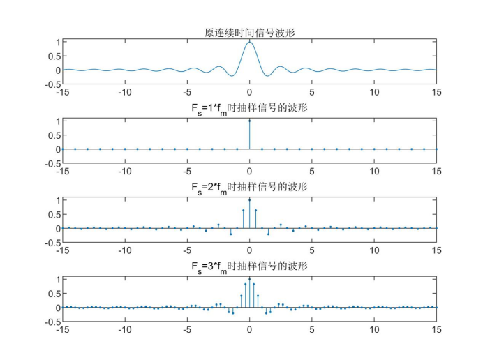
① Respectively display the waveform of the original continuous time signal and the waveform of the sampled signal under the conditions of Fs=fm, Fs=2fm and Fs=3fm;
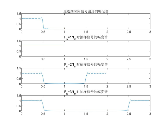
② Solving the amplitude spectrum corresponding to the original continuous signal waveform and the sampled signal;
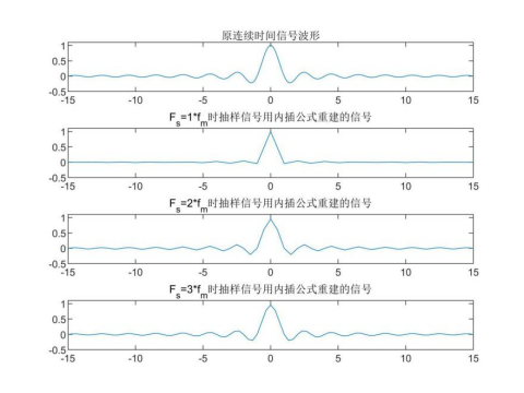
③ The time domain convolution method (interpolation formula) is used to reconstruct the signal;
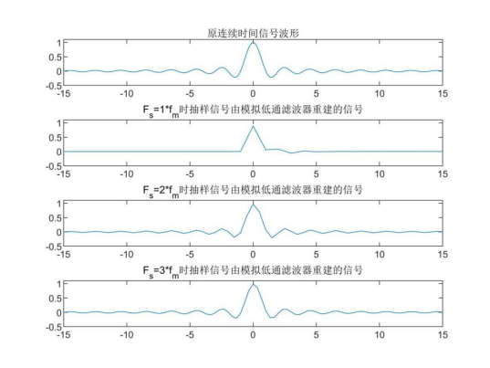
④ The signal is reconstructed with an analog low-pass filter.

In the field of digital signal processing,Therefore, it is directly generated by sinc function in matlab. When the sampling frequency is 1Hz, i.e. once per second, except when t=0, all other times are sampled at zero, so when the sampling frequency isThe waveform is 0 at all times except when t=0. Whenand The shape of the original signal can be seen on the envelope of the sampled signal.

The spectrum of sinc(t) is a rectangular window when the sampling frequencyWhen the Nyquist sampling interval is not satisfied, the signal spectrum is aliased, the spectrum of the rectangular window is just aliased into a straight line, and the response characteristic H(f)=1. Whenand When the Nyquist sampling interval is satisfied, the signal spectrum isNo aliasing occurs, and the spectrum is mirror symmetrical at.

The interpolation formula is used to reconstruct the signal, and the results are as follows:
When the sampling frequency does not meet the Nyquist interval, the reconstructed signal is obviously distorted. When the sampling frequency just meets the Nyquist interval, the curve accuracy is low, but the shape of the signal is basically recoveredThe reconstructed signal curve has high accuracy.

Reconstruct the signal using an analog filter:
The Chebyshev II low-pass filter of matlab is used to filter out the frequency part outside the limited bandwidth of the original sampling signal, and the signal can also be reconstructed. When the sampling frequency does not meet the Nyquist interval, the reconstructed signal is obviously distorted. When the sampling frequency just meets the Nyquist interval, the curve accuracy is low, but the shape of the signal is basically recoveredThe reconstructed signal curve has high accuracy, which is basically the same as the signal reconstructed by interpolation formula. It is also found that the use of Chebyshev I low-pass filter will lead to time shift of the reconstructed signal.

%question 5
clear;
dt=0.1;fm=1;
t=-15:dt:15;
f=sinc(t);   %Establish original continuous signal
figure;
subplot(4,1,1);
plot(t,f);axis([min(t) max(t) -0.5 1.1])
title('Original continuous time signal waveform');
for i=1:3
    fs=i*fm;Ts=1/fs;%Determine sampling frequency and period
    n=-15:Ts:15;
    f=sinc(n);%Generate sampling signal
    subplot(4,1,i+1);stem(n,f,'.');
    axis([min(n),max(n),-0.5,1.1]);
    title(['F_s=',num2str(i),'*f_m Waveform of time sampling signal'])
end

dt=0.1;fm=1;
t=-15:dt:15;
f=sinc(t);   %Establish original continuous signal
N=length(t);%Find the number of sampling points on the timeline
wm=2*pi*fm;
k=0:N-1;
w1=k*wm/N;%Generate on frequency axis N Sampling frequency points
F1=f*exp(-1j*t'*w1)*dt;%Fourier transform the original signal
figure;
subplot(4,1,1),plot(w1/(2*pi),abs(F1));
title('Amplitude spectrum of original continuous time signal waveform');
axis([0,3,0,1.5])
for i=1:3
    fs=i*fm;Ts=1/fs;%Determine sampling frequency and period
    n=-15:Ts:15;
    f=sinc(n);%Generate sampling signal
    N=length(n);%Find the number of sampling points on the timeline
    wm=2*pi*fs;
    k=0:N-1;
    w=k*wm/N;
    F=f*exp(-1j*n'*w)*Ts;%Fourier transform the sampled signal
    subplot(4,1,i+1);plot(w/(2*pi),abs(F));
    title(['F_s=',num2str(i),'*f_m Amplitude spectrum of time sampled signal'])
    axis([0,3,0,1.5])
end

dt=0.1;fm=1;
t=-15:dt:15;
f=sinc(t);   %Establish original continuous signal
figure;
subplot(4,1,1);
plot(t,f);axis([min(t) max(t) -0.5 1.1])
title('Original continuous time signal waveform');
for i=1:3
    fs=i*fm;
    Ts=1/fs;%Determine sampling frequency and period
    n=-15/Ts:15/Ts;
    t1=-15:Ts:15;
    f1=sinc(n/fs);%Generate sampling signal
    T_N=ones(length(n),1)*t1-n'*Ts*ones(1,length(t1));%generate t-nT matrix
    fa=f1*sinc(fs*pi*T_N);%Interpolation formula
    subplot(4,1,i+1),plot(t1,fa);
    axis([-15,15,-0.5,1.1])
    title(['F_s=',num2str(i),'*f_m Time sampled signal reconstructed by interpolation formula'])
end

dt=0.1;fm=1;
t=-15:dt:15;
f=sinc(t);   %Establish original continuous signal
figure;
subplot(4,1,1);
plot(t,f);axis([min(t) max(t) -0.5 1.1])
title('Original continuous time signal waveform');
N=6;rp=1;as=20;
for i=1:3
    fs=i*fm;
    Ts=1/fs;%Determine sampling frequency and period
    n=-15:Ts:15;
    f=sinc(n);%Generate sampling signal
    Wp=2*pi*fm;%Calculate cut-off angle frequency
    [b,a]=cheby2(N,rp,Wp,'s');%Chebyshev I type
    y=lsim(b,a,f,n);
    subplot(4,1,i+1),plot(n,y);
    axis([-15,15,-0.5,1.1])
    title(['F_s=',num2str(i),'*f_m The time sampled signal is a signal reconstructed by an analog low-pass filter'])
end

6. Topic 6

6. It is known that the spectrum of a time series is:

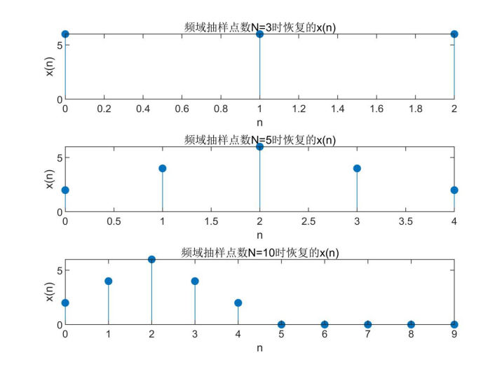
Take the frequency domain sampling points N as 3, 5 and 10 respectively, calculate and calculate the time series x(n) with IFFT, and display each time series graphically. Therefore, the condition of undistorted frequency domain sampling recovery of the original time domain signal is discussed. (answer with matlab)

The value of sampling period Ts is not given, so Ts=1 is taken. It can be seen from the spectrum expression that the time domain sequence is x(n)=[2,4,6,4,2]. As can be seen from the following images, when N=5 and N=10, the time series is not distorted, and when N=3, the time series is distorted. Therefore, the conditions for undistorted sampling and recovery of the original time domain signal from the frequency domain are as follows:
If x(n) is a finite length sequence and the number of frequency domain sampling points N is greater than or equal to the sequence length M (i.e. N ≥ M), the original signal x(n) can be recovered without distortion.

%question 6
clear;
Ts=1;%The default digital frequency is Ts=1
N0=[3,5,10];%The lengths of three spectral sequences are given N
for r=1:3
    N=N0(r);%take N value
    D=2*pi/(Ts*N);%Calculate the analog frequency resolution
    kn=floor(-(N-1)/2:-1/2);%Establish negative frequency band vector
    kp=floor(0:(N-1)/2);%Establish positive frequency band vector
    w=[kp,kn]*D;%Move the negative frequency segment to the right end of the positive frequency to form a new frequency ranking
    X=2+4*exp(-1j*w)+6*exp(-1j*2*w)+4*exp(-1j*3*w)+2*exp(-1j*4*w);
    n=0:N-1;
    x=ifft(X,N);
    subplot(3,1,r);stem(n*Ts,abs(x),'filled');
    xlabel('n');ylabel('x(n)');
    title(['Frequency domain sampling points N=',num2str(N),'Recovered at x(n)'])
end

7. Topic VII

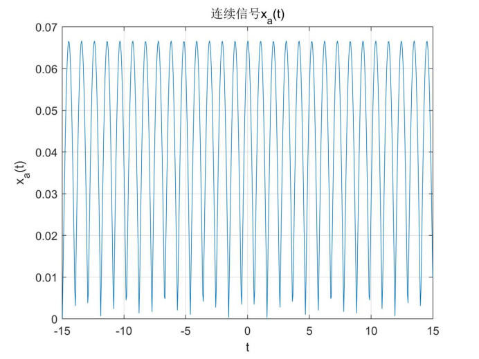
It is known that the amplitude of a spectrum in the frequency range of [- 6.28, 6.28] rad/s is 1 at the analog frequency = 3.14 and 0 in other ranges. It is required to calculate its continuous signal xa(t) and display the signal curve graphically. (answer with matlab)

The sampling frequency can be known from Nyquist sampling theorem, i.e. sampling periodWhen, aliasing will not occur. Select a smaller sampling period to increase the number of samples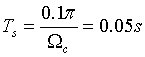. At the same time, in order to make the time signal closer to the continuous signal, the number of points N=600 is taken. The obtained continuous signal curve is as follows:
It can be concluded from the analysis that the continuous signal should be a cosine signal with a frequency of 1Hz, and the obtained continuous signal curve has slight distortion at the bottom. It is speculated that the frequency corresponding to amplitude 1 in the spectrum is caused by slight error.

%question 7
clear;
wc=6.28;
Ts=0.1*pi/wc;%The maximum sampling period is 1 of the critical value/10
N=600;
D=2*pi/(Ts*N);%Analog frequency resolution
M=floor(wc/D);%Find the subscript of the effective frequency boundary value
Xa=[zeros(1,M/2),1,zeros(1,N-M),1,zeros(1,M/2-1)];
n=-(N-1)/2:(N-1)/2;%Establish time vector
xa=abs(fftshift(ifft(Xa/Ts,N)));
plot(n*Ts,xa);
xlabel('t');ylabel('x_a(t)');
grid on;box on;
title('Continuous signal x_a(t)');