1. Topic 1
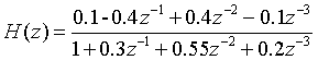
It is known that the transfer function of an IIR system is
It is converted from direct type to cascade type, parallel type and lattice structure, and the signal flow diagrams of various structures are drawn.
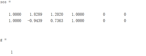
Cascade type:
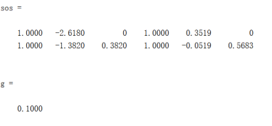
Cascaded expressions can be listed from the data of sos and g:
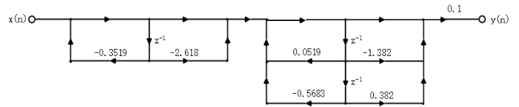
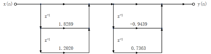
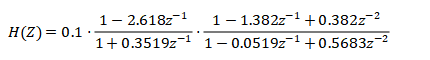 The signal flow diagram of the corresponding cascade structure is as follows:
Parallel type:
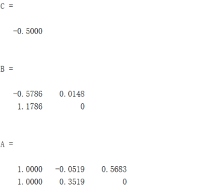
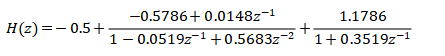
From the data of A, B and C, the expression of parallel type can be listed as follows:
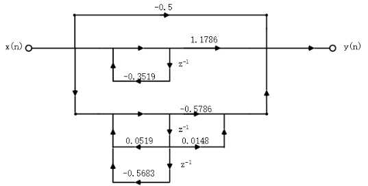
The signal flow diagram of the corresponding parallel structure is as follows:
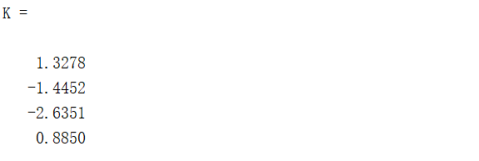
Lattice:
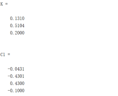
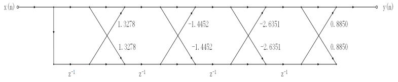
From the data of K and C1, the signal flow diagram of the corresponding lattice structure can be drawn as follows:

function [C,B,A] = dir2par(num,den)
%Direct to parallel conversion
%   Detailed description here
    M=length(num);N=length(den);
    [r,p,C]=residuez(num,den);%Find the single root of the system first p1,Corresponding residue r1 And direct items C

    %Transform to second-order subsystem
    K=floor(N/2);B=zeros(K,2);A=zeros(K,3);%Initialization of second-order subsystem variables
    if K*2==N  %N Is an even number, A(z)The number of times is odd, and there is a factor of first order
        for i=1:2:N-2
            Brow=r(i:1:i+1,:);%Take out a pair of residues
            Arow=p(i:1:i+1,:);%Take out a pair of corresponding poles
            %The two residue poles are transformed into the numerator denominator coefficients of the second-order subsystem
            [Brow,Arow]=residuez(Brow,Arow,[]);
            B(fix((i+1)/2),:)=real(Brow);
            A(fix((i+1)/2),:)=real(Arow);
        end
        [Brow,Arow]=residuez(r(N-1),p(N-1),[]);
        B(K,:)=[real(Brow),0];A(K,:)=[real(Arow),0];
    else
        for i=1:2:N-2
            Brow=r(i:1:i+1,:);%Take out a pair of residues
            Arow=p(i:1:i+1,:);%Take out a pair of corresponding poles
            %The two residue poles are transformed into the numerator denominator coefficients of the second-order subsystem
            [Brow,Arow]=residuez(Brow,Arow,[]);
            B(fix((i+1)/2),:)=real(Brow);
            A(fix((i+1)/2),:)=real(Arow);
        end
    end
end

%question 1
clear;
b=[0.1,-0.4,0.4,-0.1];%Input system function b parameter
a=[1,0.3,0.55,0.2];%Input system function a parameter
[sos,g]=tf2sos(b,a)     %Conversion from direct type to cascade type
[C,B,A]=dir2par(b,a)    %Conversion from direct type to parallel type
[K,C1]=tf2latc(b,a)      %Convert from direct type to lattice type
2. Topic 2
2. It is known that the transfer function of an FIR system is

It is transformed from cross-sectional structure to cascade and lattice structure, and the signal flow diagrams of various structures are drawn.
Cascade type:
The cascade expression can be listed from the data of sos and g as follows:

The signal flow diagram of the corresponding cascade structure is as follows:
Lattice:
The signal flow diagram of the corresponding lattice structure can be drawn from the data of K as follows:
The structure diagram is the lattice structure diagram of all zero FIR system.
%question 2
clear;
b=[1,0.885,0.212,0.212,0.885];%Input system function b parameter
a=1;%Input system function a parameter
[sos,g]=tf2sos(b,a) %Conversion from direct type to cascade type
K=tf2latc(b,1)  %Convert from direct type to lattice type
3. Topic 3
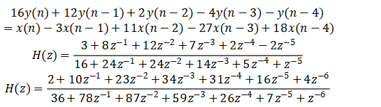
3. The equations and system functions of the three IIR filters are:
The MATLAB program is compiled to calculate the coefficients of the cascade grid of each filter and draw the cascade structure;
The MATLAB program is compiled to calculate the coefficients of the parallel grid of each filter, and draw the parallel structure.
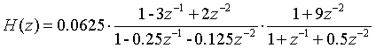
For the first IIR filter:
Cascade type:
The cascading expression can be listed from the data of sos1 and g1 as follows:
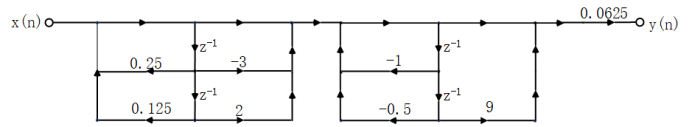
The signal flow diagram of the corresponding cascade structure is as follows:
Parallel type:
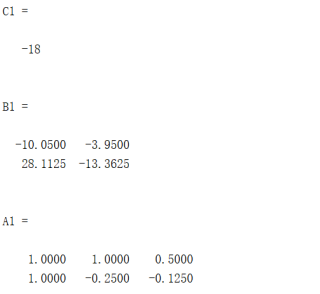
The expression of parallel type can be listed from the data of C1, B1 and A1 as follows:
The signal flow diagram of the corresponding parallel structure is as follows:
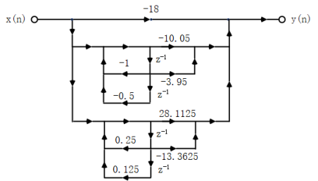
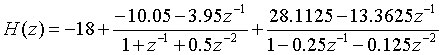
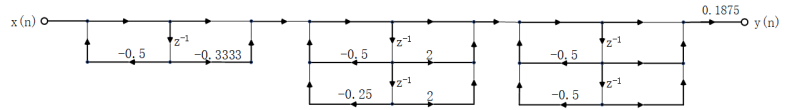
For the second IIR filter:
Cascade type:
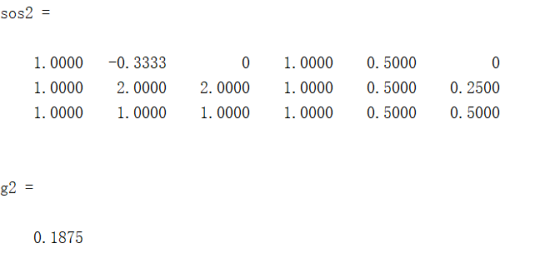
The expression of cascade type can be listed by sos2 and g2 as follows:

The signal flow diagram of the corresponding cascade structure is as follows:
Parallel type:
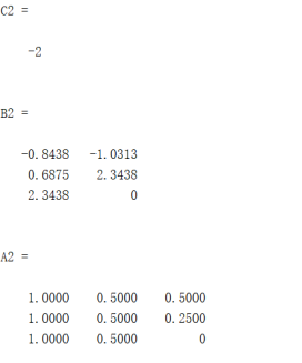
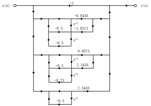
The expression of parallel type can be listed from the data of C2, B2 and A2 as follows:

The signal flow diagram of the corresponding parallel structure is as follows:
For the third IIR filter:
Cascade type:
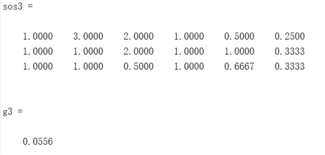
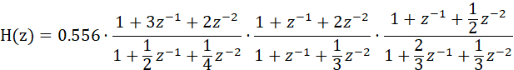
The cascading expressions listed by sos3 and g3 are:
The signal flow diagram of the corresponding cascade structure is as follows:
Parallel type:
The expression of parallel type can be listed from the data of C3, B3 and A3 as follows:

The signal flow diagram of the corresponding parallel structure is as follows:
%question 3
clear;
b1=[1,-3,11,-27,18];
a1=[16,12,2,-4,-1];
[sos1,g1]=tf2sos(b1,a1)   %Conversion from direct type to cascade type
[C1,B1,A1]=dir2par(b1,a1) %Conversion from direct type to parallel type

b2=[3,8,12,7,2,-2];
a2=[16,24,24,14,5,1];
[sos2,g2]=tf2sos(b2,a2)   %Conversion from direct type to cascade type
[C2,B2,A2]=dir2par(b2,a2) %Conversion from direct type to parallel type

b3=[2,10,23,34,31,16,4];
a3=[36,78,87,59,26,7,1];
[sos3,g3]=tf2sos(b3,a3)   %Conversion from direct type to cascade type
[C3,B3,A3]=dir2par(b3,a3) %Conversion from direct type to parallel type
4. Topic 4
An analog prototype low-pass filter is designed, with passband cut-off frequency fp=6kHz, maximum passband attenuation Rp ≤ 1dB, stopband cut-off frequency fs=15kHz and minimum stopband attenuation As ≥ 30dB. Requirements: realize Butterworth filter, Chebyshev type I filter, Chebyshev type I filter and elliptic filter that meet the above indexes respectively, draw amplitude frequency characteristic curve, phase frequency characteristic curve and zero pole distribution diagram, and write transfer function expression.
Solve with MATLAB:
Butterworth filter:
Use the MATLAB toolbox function button to calculate the order and 3dB cut-off frequency of the filter, and then use the buttap function to design the corresponding filter from the Butterworth filter prototype.
The amplitude frequency characteristic curve, phase frequency characteristic curve and zero pole distribution diagram obtained are as follows:
Show the filter coefficients a and b in polynomial form:
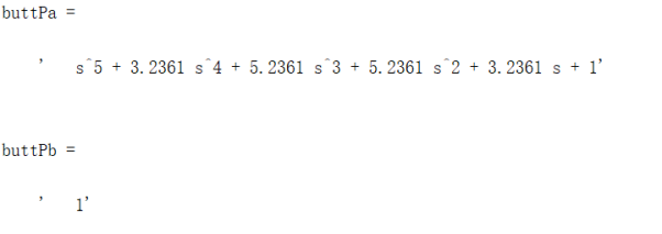
That is, the corresponding transfer function expression is:

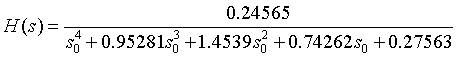
Chebyshev type I filter:
Use the MATLAB toolbox function cheb1ord to calculate the order and 3dB cut-off frequency of the filter, and then use the cheb1ap function to design the corresponding filter from the Chebyshev type I filter prototype.
The amplitude frequency characteristic curve, phase frequency characteristic curve and zero pole distribution diagram obtained are as follows:

Show the filter coefficients a and b in polynomial form:
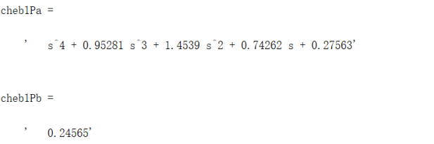
That is, the corresponding transfer function expression is:
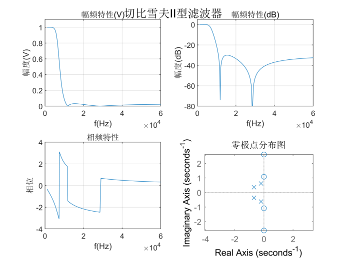
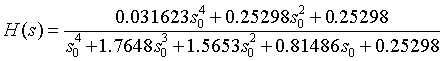
Chebyshev type II filter:
Use the MATLAB toolbox function cheb2ord to calculate the order and 3dB cut-off frequency of the filter, and then use the cheb2ap function to design the corresponding filter from the Chebyshev II filter prototype.
The amplitude frequency characteristic curve, phase frequency characteristic curve and zero pole distribution diagram obtained are as follows:
Show the filter coefficients a and b in polynomial form:
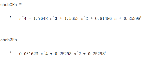
That is, the corresponding transfer function expression is:
Elliptical filter:
The order and 3dB cut-off frequency of the filter are calculated by using the MATLAB toolbox function ellipard, and then the corresponding filter is designed from the Chebyshev II filter prototype by using the ellipap function.
The amplitude frequency characteristic curve, phase frequency characteristic curve and zero pole distribution diagram obtained are as follows:
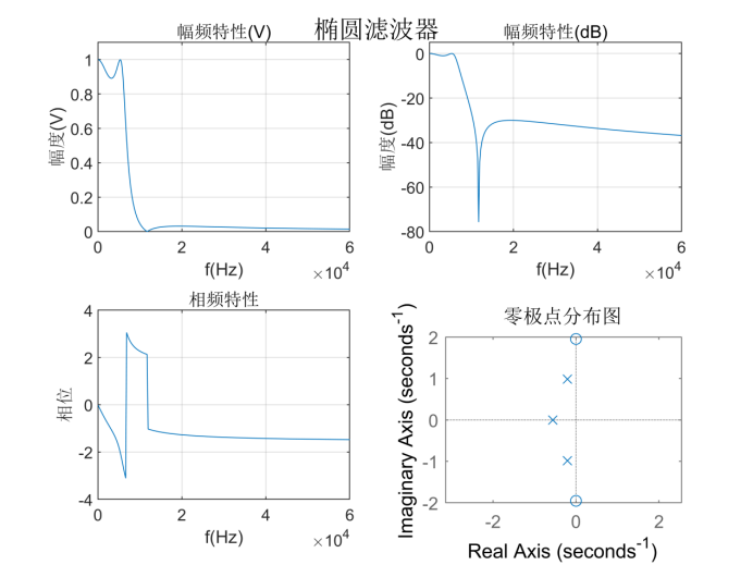
Show the filter coefficients a and b in polynomial form:
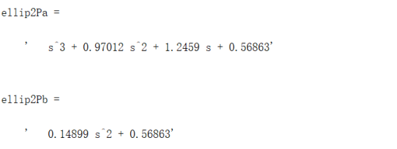
That is, the corresponding transfer function expression is:
%question 4
clear;
fp=6000;Omgp=2*pi*fp;   %Passband cut-off frequency of input filter
fs=15000;Omgs=2*pi*fs;  %Stopband cut-off frequency of input filter
Rp=1;As=30;             %Pass stop band attenuation index of input filter

%Butterworth filter
[n,Omgc]=buttord(Omgp,Omgs,Rp,As,'s');%Calculate the analog filter order and 3 dB cut-off frequency
[z0,p0,k0]=buttap(n);
b0=k0*real(poly(z0));       %Find filter coefficients b0
a0=real(poly(p0));          %Find filter coefficients a0
[H,Omg]=freqs(b0,a0);       %Find the frequency response of the system
dbH=20*log10((abs(H)+eps)/max(abs(H)));%Find the decibel value, plus eps Avoid point 0
buttPa=poly2str(a0,'s')
buttPb=poly2str(b0,'s')

figure;suptitle('Butterworth filter')
subplot(2,2,1);plot(Omg*Omgc/2/pi,abs(H));
grid on;box on;title('Amplitude frequency characteristic(V)');
axis([0,40000,0,1.1]);xlabel('f(Hz)');ylabel('range(V)');

subplot(2,2,2);plot(Omg*Omgc/2/pi,dbH);
grid on;box on;title('Amplitude frequency characteristic(dB)');
axis([0,40000,-80,5]);xlabel('f(Hz)');ylabel('range(dB)');

subplot(2,2,3);plot(Omg*Omgc/2/pi,angle(H));
grid on;box on;title('Phase frequency characteristics');
axis([0,40000,-4,4]);xlabel('f(Hz)');ylabel('phase');

subplot(2,2,4);pzmap(b0,a0);    %Draw pole zero diagram
axis square,axis equal
title('Zero pole distribution diagram')

%Chebyshev I type
[n,Omgn]=cheb1ord(Omgp,Omgs,Rp,As,'s');
[z0,p0,k0]=cheb1ap(n,Rp);
b0=k0*real(poly(z0));    %Find filter coefficients b0
a0=real(poly(p0));       %Find filter coefficients a0
b1=[zeros(1,length(a0)-length(b0)),b0];%take b0 Left end compensation 0.Make it compatible with a0 Equal length
[H,Omg]=freqs(b0,a0);   %Find the frequency response of the system
dbH=20*log10((abs(H)+eps)/max(abs(H)));
cheb1Pa=poly2str(a0,'s')
cheb1Pb=poly2str(b0,'s')

figure;suptitle('Chebyshev I Type filter')
subplot(2,2,1);plot(Omg*Omgn/2/pi,abs(H));
grid on;box on;title('Amplitude frequency characteristic(V)');
axis([0,40000,0,1.1]);xlabel('f(Hz)');ylabel('range(V)');

subplot(2,2,2);plot(Omg*Omgn/2/pi,dbH);
grid on;box on;title('Amplitude frequency characteristic(dB)');
axis([0,40000,-80,5]);xlabel('f(Hz)');ylabel('range(dB)');

subplot(2,2,3);plot(Omg*Omgn/2/pi,angle(H));
grid on;box on;title('Phase frequency characteristics');
axis([0,40000,-4,4]);xlabel('f(Hz)');ylabel('phase');

subplot(2,2,4);pzmap(b0,a0);    %Draw pole zero diagram
axis square,axis equal
title('Zero pole distribution diagram')

%Chebyshev II type
[n,Omgn]=cheb2ord(Omgp,Omgs,Rp,As,'s');
[z0,p0,k0]=cheb2ap(n,As);
b0=k0*real(poly(z0));    %Find filter coefficients b0
a0=real(poly(p0));       %Find filter coefficients a0
b1=[zeros(1,length(a0)-length(b0)),b0];%take b0 Left end compensation 0.Make it compatible with a0 Equal length
[H,Omg]=freqs(b0,a0);   %Find the frequency response of the system
dbH=20*log10((abs(H)+eps)/max(abs(H)));
cheb2Pa=poly2str(a0,'s')
cheb2Pb=poly2str(b0,'s')

figure;suptitle('Chebyshev II Type filter')
subplot(2,2,1);plot(Omg*Omgn/2/pi,abs(H));
grid on;box on;title('Amplitude frequency characteristic(V)');
axis([0,60000,0,1.1]);xlabel('f(Hz)');ylabel('range(V)');

subplot(2,2,2);plot(Omg*Omgn/2/pi,dbH);
grid on;box on;title('Amplitude frequency characteristic(dB)');
axis([0,60000,-80,5]);xlabel('f(Hz)');ylabel('range(dB)');

subplot(2,2,3);plot(Omg*Omgn/2/pi,angle(H));
grid on;box on;title('Phase frequency characteristics');
axis([0,60000,-4,4]);xlabel('f(Hz)');ylabel('phase');

subplot(2,2,4);pzmap(b0,a0);    %Draw pole zero diagram
axis square,axis equal
title('Zero pole distribution diagram')

%Elliptic filter
[n,Omgn]=ellipord(Omgp,Omgs,Rp,As,'s');
[z0,p0,k0]=ellipap(n,Rp,As);
b0=k0*real(poly(z0));    %Find filter coefficients b0
a0=real(poly(p0));       %Find filter coefficients a0
b1=[zeros(1,length(a0)-length(b0)),b0];%take b0 Left end compensation 0.Make it compatible with a0 Equal length
[H,Omg]=freqs(b0,a0);   %Find the frequency response of the system
dbH=20*log10((abs(H)+eps)/max(abs(H)));
ellip2Pa=poly2str(a0,'s')
ellip2Pb=poly2str(b0,'s')

figure;suptitle('Elliptic filter')
subplot(2,2,1);plot(Omg*Omgn/2/pi,abs(H));
grid on;box on;title('Amplitude frequency characteristic(V)');
axis([0,60000,0,1.1]);xlabel('f(Hz)');ylabel('range(V)');

subplot(2,2,2);plot(Omg*Omgn/2/pi,dbH);
grid on;box on;title('Amplitude frequency characteristic(dB)');
axis([0,60000,-80,5]);xlabel('f(Hz)');ylabel('range(dB)');

subplot(2,2,3);plot(Omg*Omgn/2/pi,angle(H));
grid on;box on;title('Phase frequency characteristics');
axis([0,60000,-4,4]);xlabel('f(Hz)');ylabel('phase');

subplot(2,2,4);pzmap(b0,a0);    %Draw pole zero diagram
axis square,axis equal
title('Zero pole distribution diagram')
5. Topic 5
5. A Chebyshev I analog low-pass filter is designed by frequency transformation method. It is required that the passband cut-off frequency fp= 3.5kHz, the maximum passband attenuation Rp ≤ 1dB, the stopband cut-off frequency fs = 6kHz, and the minimum stopband attenuation As ≥ 40dB. Draw the frequency characteristics of normalized analog filter prototype and actual analog low-pass filter.
Solve with MATLAB:
The order and 3dB cut-off frequency of the filter are calculated by cheb1ord function, and then the low-pass prototype of the analog filter is calculated by cheb1ap to obtain the normalized analog filter prototype. Then the frequency characteristics of the actual analog low-pass filter are obtained by lp2lp from the normalized low-pass to the actual low-pass.
The frequency characteristics of the normalized analog filter prototype and the actual analog low-pass filter are as follows:
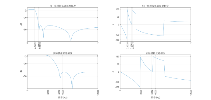
From the frequency characteristics of the normalized low-pass prototype filter and the frequency characteristics of the actual filter obtained by frequency transformation, it can be seen that the frequency characteristics of the normalized low-pass prototype and the actual filter are consistent. According to the frequency characteristic curve, the design result can meet the design index requirements of Rp ≤ 1dB and As ≥ 40dB at the cut-off frequency of pass stop band.
%question 5
clear;
fp=3500;Omgp=2*pi*fp;   %Input the passband cut-off frequency of the actual filter
fs=6000;Omgs=2*pi*fs;   %Input the stopband cut-off frequency of the actual filter
Rp=1;As=40;
[n,Omgn]=cheb2ord(Omgp,Omgs,Rp,As,'s');%Calculate the order and 3 of the filter dB cut-off frequency
[z0,p0,k0]=cheb2ap(n,As);
b0=k0*real(poly(z0));    %Find normalized filter coefficients b0
a0=real(poly(p0));       %Find normalized filter coefficients a0
[H,Omg0]=freqs(b0,a0);   %Find normalized filter frequency characteristics
dbH=20*log10((abs(H)+eps)/max(abs(H)));
[ba,aa]=lp2lp(b0,a0,Omgn);%From normalized low-pass to actual low-pass
[Ha,Omga]=freqs(ba,aa);%Find the frequency characteristics of the actual system
dbHa=20*log10((abs(Ha)+eps)/max(abs(H)));

Omg0p=fp/Omgn;      %Pass band cutoff frequency normalization
Omg0c=Omgn/2/pi/Omgn;   %3dB Cutoff frequency normalization
Omg0s=fs/Omgn;          %Stopband cutoff frequency normalization
fc=floor(Omgn/2/pi);    %3dB cut-off frequency
%Frequency characteristic mapping of normalized analog low-pass prototype
subplot(2,2,1),plot(Omg0/2/pi,dbH);
title('Normalized analog low-pass prototype amplitude');
ylabel('dB');grid on;axis([0,1,-80,5])
set(gca,'Xtick',[0,Omg0p,Omg0c,Omg0s,1]);
set(gca,'XtickLabelRotation',90);
set(gca,'Ytick',[-50,-20,-3,-1]);

subplot(2,2,2),plot(Omg0/2/pi,angle(H)/pi*180);
title('Normalized analog low-pass prototype phase');
ylabel('\phi');grid on;axis([0,1,-200,200])
set(gca,'Xtick',[0,Omg0p,Omg0c,Omg0s,1]);
set(gca,'XtickLabelRotation',90);
set(gca,'Ytick',[-180,-120,0,90,180]);

%Drawing of actual simulated low-pass frequency characteristics
subplot(2,2,3),plot(Omga/2/pi,dbHa);
title('Actual analog low pass amplitude');xlabel('frequency(Hz)')
ylabel('dB');grid on;axis([0,2*fs,-80,1])
set(gca,'Xtick',[0,fp,fc,fs,2*fs]);
set(gca,'XtickLabelRotation',90);
set(gca,'Ytick',[-50,-20,-3,-1]);

subplot(2,2,4),plot(Omga/2/pi,angle(Ha)/pi*180);
title('Actual analog low-pass phase');xlabel('frequency(Hz)')
ylabel('\phi');grid on;axis([0,2*fs,-200,200])
set(gca,'Xtick',[0,fp,fc,fs,2*fs]);
set(gca,'XtickLabelRotation',90);
set(gca,'Ytick',[-180,-120,0,90,180]);
6. Topic 6
An elliptical analog bandpass filter is designed by frequency transformation method. It is required that the cut-off frequency of passband fp1=3.5kHz, fp2=5.5kHz, the maximum attenuation Rp of passband ≤ 1dB, the cut-off frequency fs1=3kHz under stopband, the cut-off frequency fs2=6kHz above stopband and the minimum attenuation As of stopband ≥ 40dB. Draw the frequency characteristics of normalized analog filter prototype and actual analog bandpass filter.
Solve with MATLAB:
The order and 3dB cut-off frequency of the filter are obtained by using the ellipard function, and then the low-pass prototype of the analog filter is calculated by ellipap to obtain the normalized analog filter prototype. Then, the frequency characteristics of the actual analog bandpass filter are obtained by lp2bp from the normalized low-pass to the actual bandpass.
The frequency characteristics of the normalized analog filter prototype and the actual analog bandpass filter are as follows:
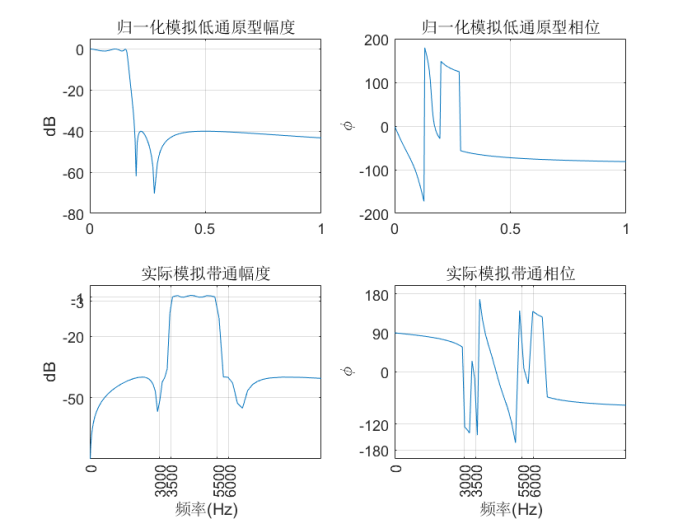
From the frequency characteristics of the normalized low-pass prototype filter and the frequency characteristics of the analog band-pass filter obtained by frequency transformation, it can be seen that the frequency characteristics of the analog band-pass filter are composed of the low-pass frequency characteristics symmetrically about the central frequency. The design results can meet the design index requirements of Rp ≤ 1dB and As ≥ 40dB at the cut-off frequency of pass stop band.
%question 6
clear;
clear;
fp1=3500;Op1=2*pi*fp1;   %The passband cut-off frequency of the input bandpass filter
fp2=5500;Op2=2*pi*fp2;
Omgp=[Op1,Op2];
fs1=3000;Os1=2*pi*fs1;  %Stopband cut-off frequency of input bandpass filter
fs2=6000;Os2=2*pi*fs2;
Omgs=[Os1,Os2];
bw=Op2-Op1;w0=sqrt(Op1*Op2);%Find the passband width and center frequency
Rp=1;As=40;                 %Pass stop band attenuation index of input filter
[n,Omgc]=ellipord(Omgp,Omgs,Rp,As,'s');%Calculate the order and 3 of the filter dB cut-off frequency
[z0,p0,k0]=ellipap(n,Rp,As);
b0=k0*real(poly(z0));    %Find normalized filter coefficients b0
a0=real(poly(p0));       %Find normalized filter coefficients a0
[H,Omg0]=freqs(b0,a0);   %Find normalized filter frequency characteristics
dbH=20*log10((abs(H)+eps)/max(abs(H)));
[ba,aa]=lp2bp(b0,a0,w0,bw);%From normalized low-pass to analog bandpass
[Ha,Omga]=freqs(ba,aa);%Find the frequency characteristics of the actual system
dbHa=20*log10((abs(Ha)+eps)/max(abs(H)));

%Frequency characteristic mapping of normalized analog low-pass prototype
subplot(2,2,1),plot(Omg0/2/pi,dbH);
title('Normalized analog low-pass prototype amplitude');
ylabel('dB');grid on;axis([0,1,-80,5])

subplot(2,2,2),plot(Omg0/2/pi,angle(H)/pi*180);
title('Normalized analog low-pass prototype phase');
ylabel('\phi');grid on;axis([0,1,-200,200])

%Drawing of actual simulated low-pass frequency characteristics
subplot(2,2,3),plot(Omga/2/pi,dbHa);
title('Actual analog bandpass amplitude');xlabel('frequency(Hz)')
ylabel('dB');grid on;axis([0,10000,-80,5])
set(gca,'Xtick',[0,fs1,fp1,fp2,fs2]);
set(gca,'XtickLabelRotation',90);
set(gca,'Ytick',[-50,-20,-3,-1]);

subplot(2,2,4),plot(Omga/2/pi,angle(Ha)/pi*180);
title('Actual analog bandpass phase');xlabel('frequency(Hz)')
ylabel('\phi');grid on;axis([0,10000,-200,200])
set(gca,'Xtick',[0,fs1,fp1,fp2,fs2]);
set(gca,'XtickLabelRotation',90);
set(gca,'Ytick',[-180,-120,0,90,180]);