1 Introduction

Similarity and dissimilarity are important concepts in machine learning, because they are adopted by many data mining technologies, such as common clustering, nearest neighbor classification and anomaly detection. In many cases, once we calculate the similarity or dissimilarity of eigenvectors, we no longer need the original data. Such methods usually transform the data into similarity (dissimilarity) space, and then do data analysis.

2 Definition

• Similarity: a numerical measure of the degree of similarity between two objects. The more similar two objects are, the higher their similarity is; The value is usually non negative, usually between [0,1].
• Dissimilarity: a numerical measure of the degree of difference between two objects. The more similar the two objects are, the lower the value is. Usually, the value is non negative, the minimum dissimilarity is 0, and the upper bound is uncertain. The term distance is usually used as a synonym for dissimilarity, and distance is often used to represent a specific type of dissimilarity. This paper focuses on the common dissimilarity measurement functions.

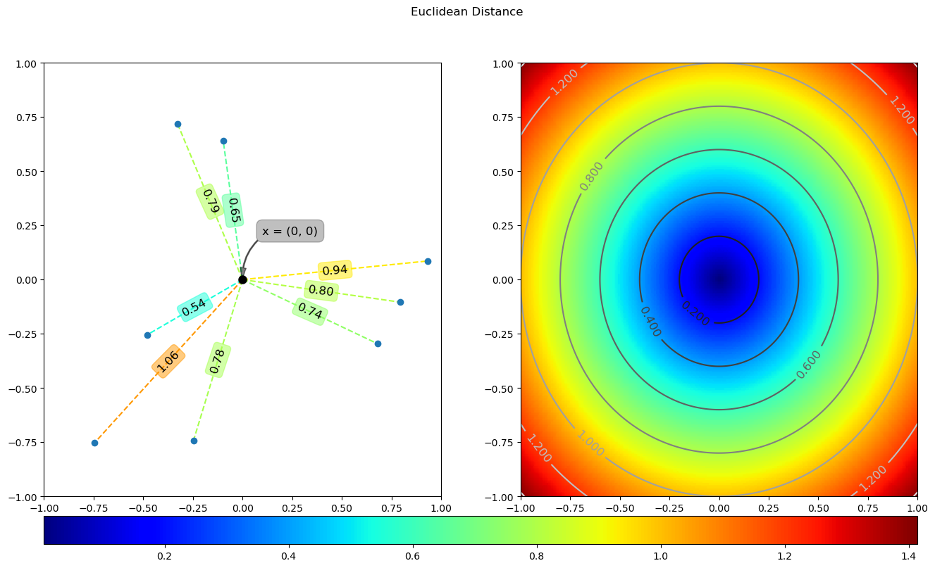
3 Euclidean distance

Euclidean distance is the most understandable distance calculation method, which comes from the distance formula between two points in Euclidean space. The calculation formula is as follows:

The code is as follows:

import numpy as np
from dissimilarity__utils import *

def test_euclidean():
    eucl = lambda x, y: np.sum((x - y)**2, axis=1)**0.5
    x = np.array([0, 0])
    dA = eucl(x, yA)
    dB = eucl(x, yB).reshape(s.shape)
    plotDist(x, dA, dB, 'euclidean_distance', save=True)

The values of yA and yB are in dissimilarity_utils is defined as follows:

r = 1
np.random.seed(123456)
y1A = np.random.uniform(-r, r, 8)
y2A = np.random.uniform(-r, r, 8)
yA = np.array([y1A, y2A]).T
M, N = 32j, 32j
s, t = np.mgrid[-r:r:N*8, -r:r:M*8]
yB = np.array([s.ravel(), t.ravel()]).T

The running results of the above code are as follows:

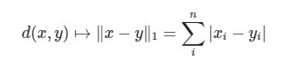
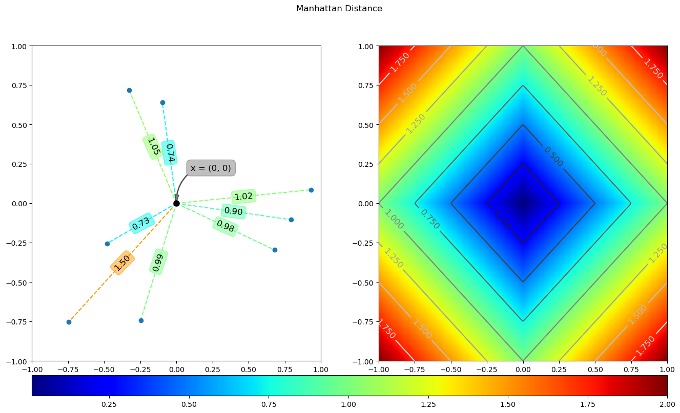
4 Manhattan distance

Manhattan distance is calculated as follows:

The code implementation is as follows:

def test_manhattan():
    manh = lambda x, y: np.sum(np.absolute(x - y), axis=1)
    x = np.array([0, 0])
    dA = manh(x, yA)
    dB = manh(x, yB).reshape(s.shape)
    plotDist(x, dA, dB, 'manhattan_distance', save=True)

The running results of the above code are as follows:

5 Chebyshev distance

Have you ever played chess? The king can move to any of the eight adjacent squares in one step. So how many steps does it take for the king to go from grid (x1,y1) to grid (x2,y2)? Try walking by yourself. You will find that the minimum number of steps is always max (| x2-x1 |, | y2-y1 |) steps. A similar distance measure is called Chebyshev distance. The calculation formula is as follows:

The code implementation is as follows:

def test_chebyshev():
    cheb = lambda x, y: np.max(np.absolute(x - y), axis=1)
    x = np.array([0, 0])
    dA = cheb(x, yA)
    dB = cheb(x, yB).reshape(s.shape)
    plotDist(x, dA, dB, 'chebyshev_distance', save=True)

The running results of the above code are as follows:

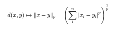
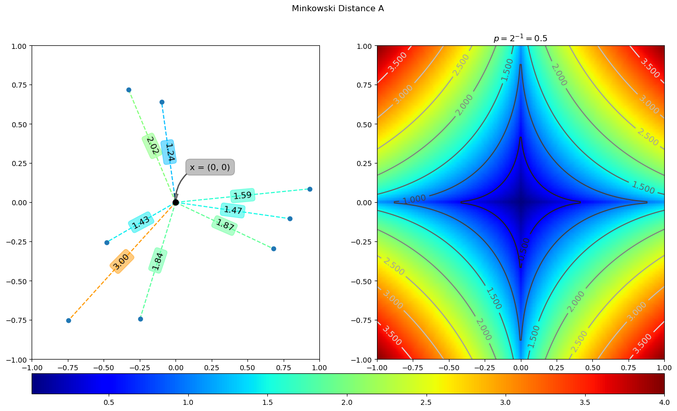
6 Minkowski distance

Min's distance is not a distance, but a definition of a set of distances. The calculation formula is as follows:

The code implementation is as follows:

def test_minkowski():
    mink = lambda x, y, p: np.sum(np.absolute(x - y) ** p, axis=1) ** (1 / p)
    x = np.array([0, 0])
    p = 2 ** -1
    dA = mink(x, yA, p)
    dB = mink(x, yB, p).reshape(s.shape)
    plotDist(x, dA, dB, 'minkowski_distance_A', ctitle=r'$p=2^{0}{2}{1}={3}$'.format('{', '}', -1, p), save=True)

The running results of the above code are as follows:

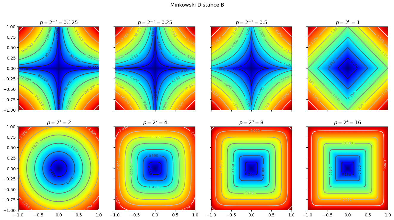
We can set different p values to compare the results under different p values. The code is as follows:

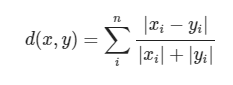
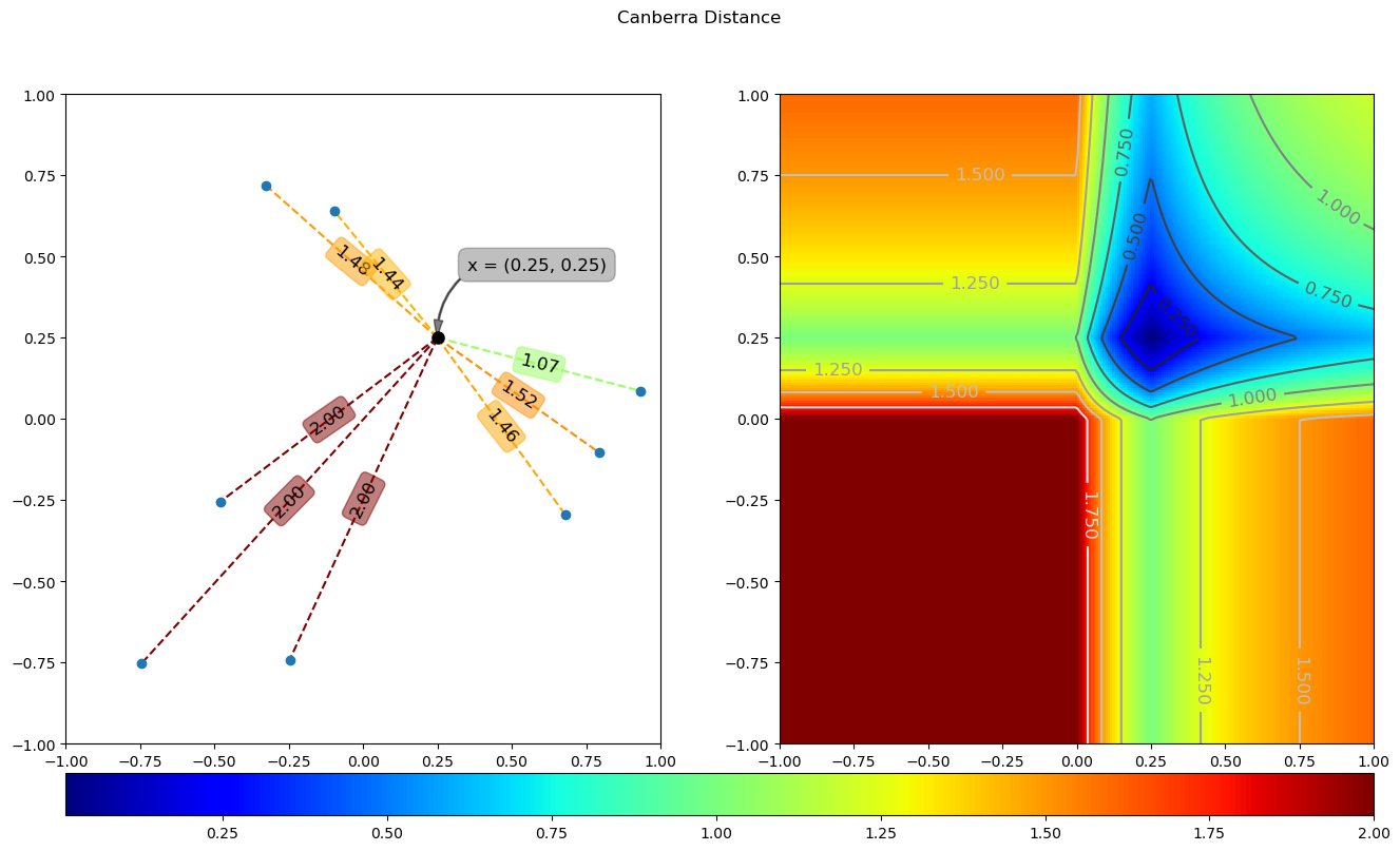
7 Canberra distance

Canberra distance can be a weighted version of Manhattan distance, and its calculation formula is as follows:

The code implementation is as follows:

def canb(x, y):
    num = np.absolute(x - y)
    den = np.absolute(x) + np.absolute(y)
    return np.sum(num/den, axis = 1)

def test_canberra():
    x = np.array([0.25, 0.25])
    dA = canb(x, yA)
    dB = canb(x, yB).reshape(s.shape)
    plotDist(x, dA, dB, 'canberra_distance', save=True)

The running results of the above code are as follows:

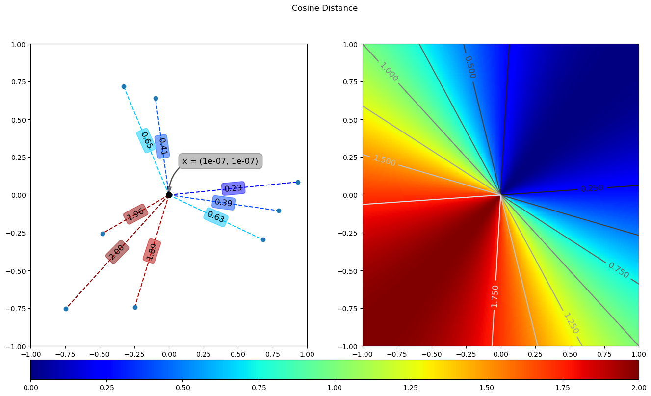
8 included angle cosine distance

The angle cosine in geometry can be used to measure the difference between the directions of two vectors. This concept is borrowed in machine learning to measure the difference between sample vectors. The calculation formula is as follows:

The code implementation is as follows:

def coss(x, y):
    if x.ndim == 1:
        x = x[np.newaxis]
    num = np.sum(x*y, axis=1)
    den = np.sum(x**2, axis = 1)**0.5
    den = den*np.sum(y**2, axis = 1)**0.5
    return 1 - num/den

def test_cosine():
    x = np.array([1e-7, 1e-7])
    dA = coss(x, yA)
    dB = coss(x, yB).reshape(s.shape)
    plotDist(x, dA, dB, 'cosine_distance', save=True)

The running results of the above code are as follows:

9 summary

This paper focuses on the calculation formulas of the similarity and dissimilarity of feature vectors in the field of machine learning, gives the common distance calculation formulas and code implementation, and gives the diagrams of different distances, which is convenient for children's shoes to understand intuitively.

Have you failed in your studies?

10 appendix

The reference links of this article are as follows:

Link one

Link 2

Pay attention to the official account of AI algorithm and get more AI algorithm information.

Note: complete code, pay attention to official account, background reply * * distance *, you can get it.