Reference link:
https://mofanpy.com/tutorials/machine-learning/reinforcement-learning/intro-q-learning/
Chapter 2 Q-learning
Reinforcement learning is a famous algorithm, Q-learning. As can be seen from the first chapter, the classification of Q-learning is model free, based on value, one-step update and offline learning.
2.1 what is Q-Learning
2.1.1 code of conduct
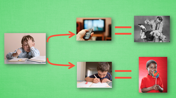
We all have our own code of conduct. For example, when we were young, our parents often said, "don't watch TV until we finish our homework". So when we are doing our homework, the good behavior is to continue to do our homework until we finish it. We can also be rewarded. The bad behavior is to watch TV before we finish it. When our parents find out, the consequences are very serious. When we were young, this kind of thing became our indelible memory. What does this have to do with Q learning? It turns out that Q learning is also a decision-making process, which is similar to that in childhood. We give examples
Suppose we are in the state of doing our homework, and we haven't tried to watch TV while doing our homework before, so now we have two choices: 1. Continue to do our homework, 2. Run to watch TV. Because we haven't been punished before, I choose to watch TV, and then the current state becomes watching TV. I choose to continue watching TV, then I still watch TV, and finally my parents go home, I found that I went to watch TV before finishing my homework, which severely punished me once. I also deeply wrote down this experience, and changed the behavior of "watching TV before finishing my homework" into a negative behavior in my mind. Let's see how Q learning makes decisions based on many such experiences.
2.1.2 QLearning decision
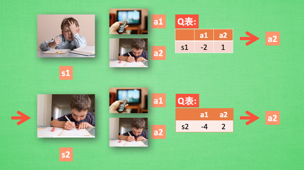
Assuming that our code of conduct has been learned well, now we are in state s1. I am doing my homework. I have two behaviors a1 and a2, respectively watching TV and doing my homework. According to my experience, in this s1 state, the potential reward brought by a2 doing my homework is higher than that of a1 watching TV (compare the value of different decisions), The potential reward here can be replaced by a Q table about s and A. in my memory, Q(s1, a1)=-2 is less than Q(s1, a2)=1, so we judge to choose a2 as the next behavior. Now our status is updated to s2. We still have two same choices. Repeat the above process, find the values of Q(s2, a1) and Q(s2, a2) in the code of conduct Q table, compare their sizes, and select the larger one. Then, according to a2, we reach s3 and repeat the above decision-making process here. The method of Q learning is just like this. After reading the decision-making, I'll study how this code of conduct Q table is changed and improved.
2.1.3 QLearning update
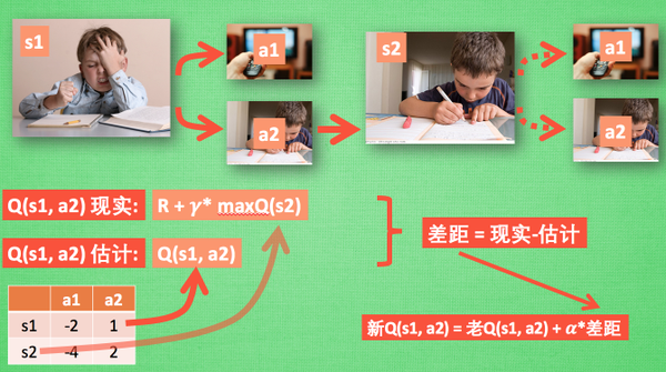
So let's go back to the previous process. According to the estimation of Q table, because the value of a2 in s1 is relatively large, through the previous decision-making method, we take a2 in s1 and reach s2. At this time, we start to update the Q table for decision-making. Then we don't take any behavior in practice, but imagine that we have taken each behavior on s2, Take a look at which of the two behaviors has a larger Q value. For example, the value of Q(s2, a2) is larger than that of Q(s2, a1), so we multiply the larger Q(s2, a2) by a attenuation value gamma (for example, 0.9) and add the reward R obtained when reaching s2 (our lollipop has not been obtained here, so the reward is 0), because we will obtain a real reward R, We take this as the value of Q(s1, a2) in my reality, but we estimated the value of Q(s1, a2) according to the Q table. Therefore, with the reality and estimated value, we can update Q(s1, a2). According to the gap between the estimation and reality, multiply the gap by a learning efficiency alpha, and accumulate the old value of Q(s1, a2) to become a new value. But always remember that although we have estimated the s2 state with maxQ(s2), we have not made any behavior in s2. The behavior decision of s2 should be made again after the update. This is how off policy Q learning makes decisions and learns to optimize decisions.
2.1.4 overall qlearning algorithm
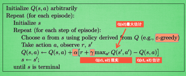
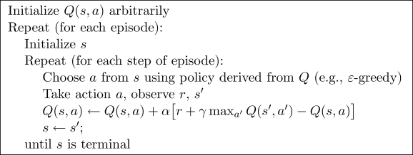
This picture summarizes all our previous content. This is also the algorithm of Q learning. We use Q reality and Q estimation for each update, and the charm of Q learning is that in Q(s1, a2) reality, it also contains a maximum estimate of Q(s2). It is wonderful to take the maximum estimate of the attenuation in the next step and the current reward as the reality of this step. Finally, let's talk about the significance of some parameters in this algorithm. Epsilon grey is a strategy used in decision-making. For example, when epsilon = 0.9, it means that I will select the behavior according to the optimal value of Q table in 90% of the cases, and use the random selection behavior in 10% of the time. alpha is the learning rate to determine how many errors are to be learned this time. alpha is a number less than 1. gamma is the attenuation value for future reward.
2.1.5 Gamma in qlearning
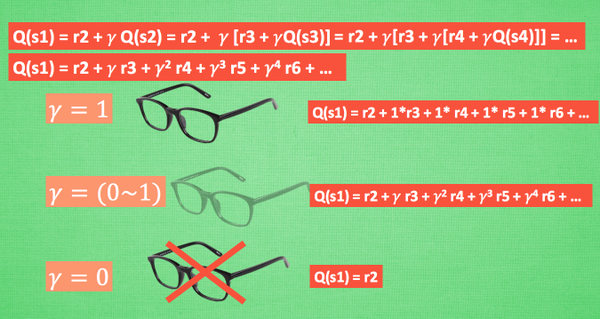
Let's rewrite the formula of Q(s1) and take Q(s2) apart, because Q(s2) can be about Q(s3) like Q(s1), so it can be written like this, and so on. Keep writing like this, and finally it can be written like this. It can be seen that Q(s1) is related to all subsequent rewards, but these rewards are decaying. The farther away from s1, the more serious the state decays. Hard to understand? OK, let's imagine that the robot of Qlearning is naturally short-sighted. When gamma = 1, the robot has a pair of appropriate glasses. The Q seen in s1 is the reward that there is no decay in the future, that is, the robot can clearly see the full value of all subsequent steps, but when gamma =0, the short-sighted robot can only touch the reward in front of it without glasses, Similarly, it only cares about the recent big reward. If gamma changes from 0 to 1, the degree of glasses changes from shallow to deep, and the more clearly it sees the value in the distance, so the robot gradually becomes far sighted, not only looking at the immediate interests, but also thinking about its own future.
2.1.6 supplement
1. Why not directly update the old Q value with the real value?
Q value is the cumulative variable of future development, not only the actual value of the next step
The definition of Q value starts from the current state, and then each state decision takes the optimal solution until the action quality of the last state (Game over).
Q value can see through the future at a glance, which is the charm of Q-learning.
Reward table R is naturally generated and exists objectively.
2.2 small examples
2.2.1 key points
This time, we will use tabular Q-learning to realize a small example. The environment of the example is a one-dimensional world. There are treasures on the right side of the world. As long as the Explorer gets the treasure, he will taste the sweetness, and then remember the method to get the treasure. This is the behavior he learned with reinforcement learning.
-o---T
# T is the location of the treasure and o is the location of the explorer
Q-learning is a method of recording behavior value. Each behavior in a certain state will have a value Q(s, a), that is, the value of behavior a in s state is Q(s, a). In the Explorer game above, s is where o is. The Explorer at each location can make two actions left/right, which is all the feasible a of the explorer.
If the Explorer calculates two behaviors he can have at a certain location s1, a1/a2=left/right, and the calculation result is Q (s1, A1) > Q (s1, A2), the Explorer will choose the behavior of left. This is the simple rule of behavior selection of Q learning.
Of course, we will elaborate on more specific rules. In the following tutorials, we will explain various methods in RL in more detail. Just look at the following contents. Just have a general RL concept and know some key steps of RL. There is no need to study the algorithms in this section carefully.
2.2.2 preset values
Module and parameter settings required this time:
import numpy as np
import pandas as pd
import time

N_STATES = 6   # Width of 1D world
ACTIONS = ['left', 'right']     # Searcher's available actions
EPSILON = 0.9   # greedy
ALPHA = 0.1     # Learning rate
GAMMA = 0.9    # Diminishing value of reward
MAX_EPISODES = 13   # Maximum rounds
FRESH_TIME = 0.3    # Movement interval
2.2.3 form Q
For tabular Q learning, we must put all Q values in Q_ In table, update q_table is also updating his code of conduct. q_ The index of table is all corresponding state s (explorer location), and columns is the corresponding action (explorer behavior).
def build_q_table(n_states, actions):
    table = pd.DataFrame(
        np.zeros((n_states, len(actions))),     # q_table all 0 initial
        columns=actions,    # columns corresponds to the behavior name
    )
    return table

# q_table:
"""
   left  right
0   0.0    0.0
1   0.0    0.0
2   0.0    0.0
3   0.0    0.0
4   0.0    0.0
5   0.0    0.0
"""
2.2.4 define actions
Then define how the Explorer selects the behavior. This is the concept of epsilon greedy we introduced. Because in the initial stage, the random exploration environment is often better than the fixed behavior pattern, so this is also the stage of accumulating experience. We hope the Explorer will not be so greedy. So EPSILON is the value used to control the degree of greed. EPSILON can increase with the exploration time (more and more greedy), but in this example, we fixed EPSILON = 0.9, 90% of the time is to select the optimal strategy, and 10% of the time is to explore.
# At a state location, select the behavior
def choose_action(state, q_table):
    state_actions = q_table.iloc[state, :]  # Select all action values of this state
    if (np.random.uniform() > EPSILON) or (state_actions.all() == 0):  # Non greedy or this state has not been explored
        action_name = np.random.choice(ACTIONS)
    else:
        action_name = state_actions.argmax()    # Greedy model
    return action_name
2.2.5 environmental feedback S_, R
After the behavior is made, the environment should also give us a feedback on our behavior, and feedback the reward (R) obtained by making action (A) in the next state (S) and the last state (S). The rule defined here is that only when o moves to T, the Explorer will get the only reward. The reward value R=1, and there is no reward in other cases.
def get_env_feedback(S, A):
    # This is how agent will interact with the environment
    if A == 'right':    # move right
        if S == N_STATES - 2:   # terminate
            S_ = 'terminal'
            R = 1
        else:
            S_ = S + 1
            R = 0
    else:   # move left
        R = 0
        if S == 0:
            S_ = S  # reach the wall
        else:
            S_ = S - 1
    return S_, R
2.2.6 environment update
The next step is to update the environment. Don't look closely.
def update_env(S, episode, step_counter):
    # This is how environment be updated
    env_list = ['-']*(N_STATES-1) + ['T']   # '---------T' our environment
    if S == 'terminal':
        interaction = 'Episode %s: total_steps = %s' % (episode+1, step_counter)
        print('\r{}'.format(interaction), end='')
        time.sleep(2)
        print('\r                                ', end='')
    else:
        env_list[S] = 'o'
        interaction = ''.join(env_list)
        print('\r{}'.format(interaction), end='')
        time.sleep(FRESH_TIME)
2.2.7 main cycle of reinforcement learning
The most important place is here. The RL methods you define are reflected here. In the following tutorial, we will explain various methods in RL in more detail. You can have a general look at the following contents. There is no need to study this section carefully.

def rl():
    q_table = build_q_table(N_STATES, ACTIONS)  # Initial q table
    for episode in range(MAX_EPISODES):     # round
        step_counter = 0
        S = 0   # Initial position of turn
        is_terminated = False   # End of turn
        update_env(S, episode, step_counter)    # Environment update

        while not is_terminated:
            A = choose_action(S, q_table)   # Selective behavior
            S_, R = get_env_feedback(S, A)  # Implement actions and get feedback from the environment
            q_predict = q_table.loc[S, A]    # Estimated (state behavior) value
            if S_ != 'terminal':
                q_target = R + GAMMA * q_table.iloc[S_, :].max()   #  Actual (status behavior) value (round not over)
            else:
                q_target = R     #  Actual (status behavior) value (end of turn)
                is_terminated = True    # terminate this episode

            q_table.loc[S, A] += ALPHA * (q_target - q_predict)  #  q_table update
            S = S_  # The Explorer moves to the next state

            update_env(S, episode, step_counter+1)  # Environment update

            step_counter += 1
    return q_table
After writing all the evaluation and update guidelines, we can start training. Throw the Explorer into the environment and let it play by itself.
if __name__ == "__main__":
    q_table = rl()
    print('\r\nQ-table:\n')
    print(q_table)
2.2.8 supplement
1. Run to Q_ predict = q_ A KeyError occurred in table.loc [S, a].
Solution: put action_ name = state_ Change actions. Argmax() to action_name = ACTIONS[state_actions.argmax()].
2.3 Q-learning algorithm update
2.3.1 key points
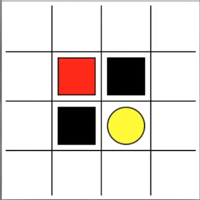
Last time we learned what the Q-learning method in RL is doing. Today we will talk about a more specific example. Let the Explorer learn to walk the maze. Yellow is heaven (reward 1), black is hell (reward -1). Most RLS are guided by reward, so defining reward is an important point in RL.
2.3.2 algorithm
The whole algorithm is to constantly update the value in Q table, and then judge what action to take in a state according to the new value. Qlearning is an off policy algorithm, because the max action in it allows the update of Q table not to be based on the experience being experienced (it can be learning the experience of a long time ago or even the experience of others). However, in this example, we did not apply off policy, but applied qlearning to on policy, that is, learn and sell now, and directly learn and apply what we have experienced on the spot.
2.3.3 code form of algorithm
First, we import two modules, maze_env is our environment module, which has been written. You can directly Download here , maze_env module we don't need to study in depth. If you are interested in editing environment, you can see how to use python's own simple GUI module tkinter to write virtual environment. I also have Corresponding tutorial . maze_env is written in tkinter. RL_ The brain module is the brain part of RL, which we will talk about in the next section.
from maze_env import Maze
from RL_brain import QLearningTable
The following code can be mapped according to the algorithm in the above picture. This is the most important iterative update part of the whole Qlearning.
def update():
    # Learn 100 rounds
    for episode in range(100):
        # Initialize state observations
        observation = env.reset()

        while True:
            # Update visual environment
            env.render()

            # RL brain selects action according to the observed value of state
            action = RL.choose_action(str(observation))

            # The Explorer implements this action in the environment and obtains the next state observation value returned by the environment, reward and done (whether it is falling into hell or going to heaven)
            observation_, reward, done = env.step(action)

            # RL learns from this sequence (state, action, reward, state_)
            RL.learn(str(observation), action, reward, str(observation_))

            # Pass the value of the next state to the next loop
            observation = observation_

            # If you fall into hell or go to heaven, this round is over
            if done:
                break

    # End the game and close the window
    print('game over')
    env.destroy()

if __name__ == "__main__":
    # Define environment env and RL mode
    env = Maze()
    RL = QLearningTable(actions=list(range(env.n_actions)))

    # Start visualizing environment env
    env.after(100, update)
    env.mainloop()
2.3.4 supplement
1. Why does the red box walk sideways during training?
It should be the frame skipping problem of tkinter. In fact, it has taken two steps
2. The initial value of observation (5, 5, 35, 35) corresponds to the understandable coordinates (x,y). How should this be converted?
Is the x1,y1,x2,y2 coordinates of the square.
3. Hello, I see maze_ In the env code, you don't see the restrictions on action s for different state s.
For example, when you have reached the boundary of maze, don't you need to limit the behavior of the box? After running run this, it is found that the movement refresh rate of the box at the boundary is not always the same. Is it because the above action s are not limited?
In maze_ Line 95 of env.py is limited.
if action == 0:
    if s[1] > UNIT:
        base_action[1] -= UNIT
elif action == 1:
    if s[1] < (MAZE_H - 1) * UNIT:
        base_action[1] += UNIT
elif action == 2:
    if s[0] < (MAZE_W - 1) * UNIT:
        base_action[0] += UNIT
elif action == 3:
    if s[0] > UNIT:
        base_action[0] -= UNIT
However, on the action output of rl, there are no restrictions on the up, down, left and right actions.
2.4 Q-learning thinking and decision-making
2.4.1 code main structure
The difference from the last time is that we will define Q learning in the form of a class and call this tabular q learning method QLearningTable.
class QLearningTable:
    # initialization
    def __init__(self, actions, learning_rate=0.01, reward_decay=0.9, e_greedy=0.9):

    # Selective behavior
    def choose_action(self, observation):

    # Learn to update parameters
    def learn(self, s, a, r, s_):

    # Check whether state exists
    def check_state_exist(self, state):
2.4.2 preset values
import numpy as np
import pandas as pd


class QLearningTable:
    def __init__(self, actions, learning_rate=0.01, reward_decay=0.9, e_greedy=0.9):
        self.actions = actions  # a list
        self.lr = learning_rate # Learning rate
        self.gamma = reward_decay   # Reward attenuation
        self.epsilon = e_greedy     # greediness
        self.q_table = pd.DataFrame(columns=self.actions, dtype=np.float64)   # Initial q_table
2.4.3 decision behavior
Here is the definition of how to make decisions according to the state or observation on the state.
def choose_action(self, observation):
        self.check_state_exist(observation) # Check whether this state is in q_table exists (see the following title)

        # Select action
        if np.random.uniform() < self.epsilon:  # Select the action with the highest Q value
            state_action = self.q_table.loc[observation, :]

            # There may be multiple Q action value s in the same state, so let's order them out of order
            action = np.random.choice(state_action[state_action == np.max(state_action)].index)

        else:   # Randomly select action
            action = np.random.choice(self.actions)

        return action
2.4.4 learning
As in the previous simple q learning example, we judge how to change Q according to whether it is a terminal state_ Table. Are you familiar with the update method:
update = self.lr * (q_target - q_predict)
This can be understood as the update mode of neural network, learning rate * (real value - predicted value). Passing back the judgment error is similar to the update of neural network.
def learn(self, s, a, r, s_):
        self.check_state_exist(s_)  # Detection Q_ Whether s exists in table_ (see the following title)
        q_predict = self.q_table.loc[s, a]
        if s_ != 'terminal':
            q_target = r + self.gamma * self.q_table.loc[s_, :].max()  # The next state is not a terminator
        else:
            q_target = r  # The next state is the terminator
        self.q_table.loc[s, a] += self.lr * (q_target - q_predict)  # Update the corresponding state action value
2.4.5 check whether the state exists
This function is to detect Q_ If there is no current state in the table, we will insert a set of all 0 data as the initial values of all action s of the state.
def check_state_exist(self, state):
        if state not in self.q_table.index:
            # append new state to q table
            self.q_table = self.q_table.append(
                pd.Series(
                    [0]*len(self.actions),
                    index=self.q_table.columns,
                    name=state,
                )
            )