about
Yesterday I read a high-quality Python topographic map blog. With emotion, I thought of the characteristics of GEE (Google earth engine) with many data sources, fast calculation speed and many calculation operators. Using GEE should not be inferior to python.
Production process
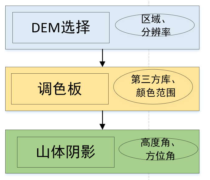
There are three steps to draw DEM with GEE, the most important of which is the use of palette.
(1) DEM data source
There are many DEM data in GEE. Readers can choose the appropriate data source according to their own needs. The study area is large, so you can choose the data with low resolution. If the study area is small, try to use high-resolution DEM.
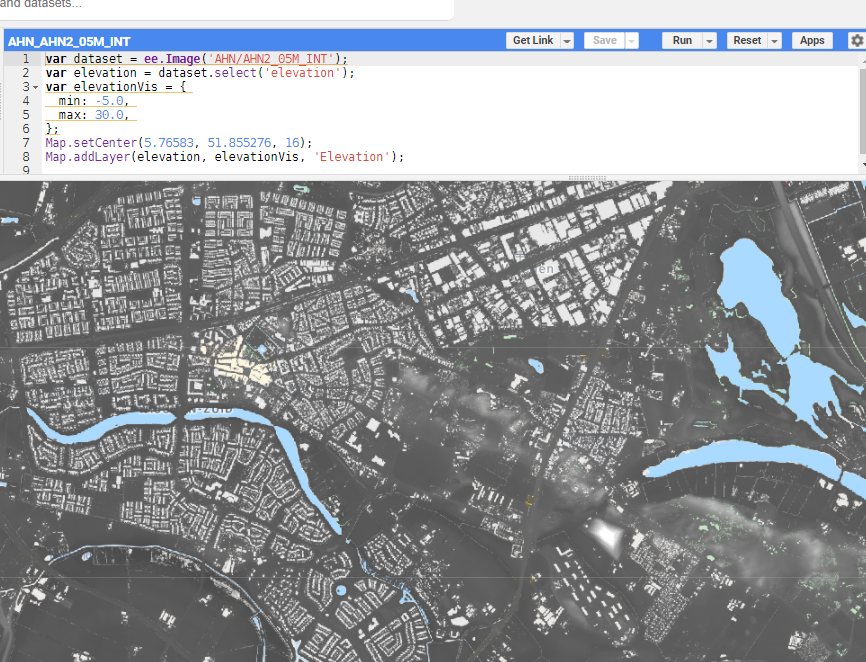
Each data source in GEE has detailed introduction and code reference examples, such as 0.5m resolution DEM in the Netherlands:
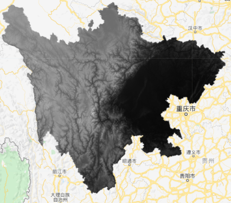
Considering that the test area is my hometown in Sichuan Province, NASA DEM with 30m resolution covering the world is used here.
// Introduce data source and select my hometown Sichuan Province as the research area
var dataset = ee.Image('NASA/NASADEM_HGT/001');
var elevation = dataset.select('elevation').clip(ROI);
// Set visualization parameters
var elevationVis = {
  min: 0,
  max: 8000,
};
//visualization
Map.addLayer(elevation, elevationVis, 'Elevation');
Map.centerObject(ROI, 7);
(2) Color matching table
After the data is loaded, the color of the data is not good-looking. At this time, you need a palette. There are several methods. One is to manually adjust the DEM display in GEE:

Another is that you can refer to other people's already set palettes and call them directly. Here I recommend a GitHub warehouse EE palettes( https://github.com/gee-community/ee-palettes ):
The warehouse collects nearly 200 color schemes, which can be directly called in GEE:
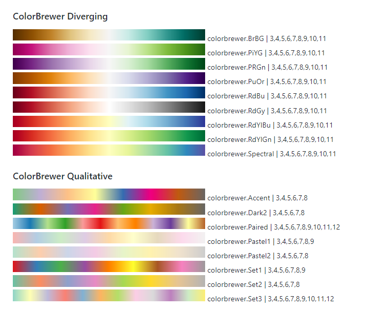
To call this warehouse, you only need to introduce the function library, then create a new palette, fill the color scheme into the map loading function, and pay attention to setting the maximum and minimum values. Then try one by one against the color table to find the most suitable color scheme.
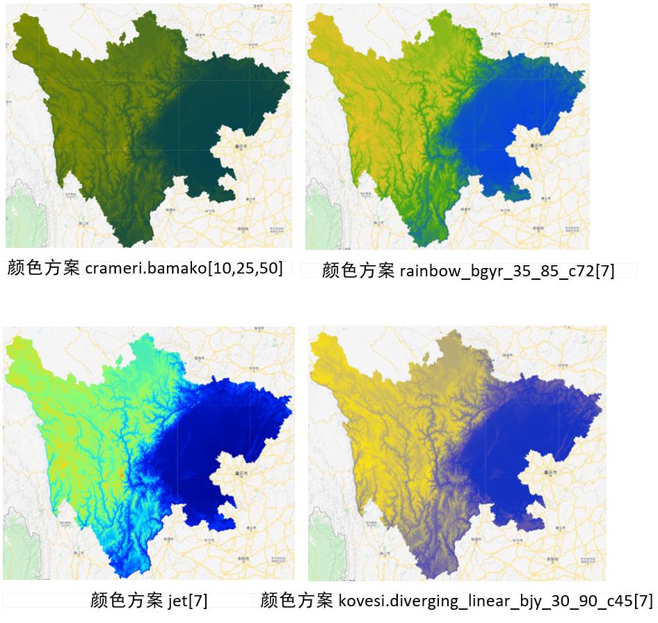
//Call the palette that has been configured in the warehouse
var palettes = require('users/gena/packages:palettes');

var palette_bamako = palettes.crameri.bamako[10,25,50];
Map.addLayer(elevation, {min:0, max:8000, palette: palette_bamako},  'crameri.bamako');

var palette_rainbow = palettes.kovesi.rainbow_bgyr_35_85_c72[7];
Map.addLayer(elevation, {min:0, max:8000, palette: palette_rainbow},  'palette_rainbow');

var palette_misc = palettes.misc.jet[7];
Map.addLayer(elevation, {min:0, max:8000, palette: palette_misc},  'palette_misc');

var palette_diverging = palettes.kovesi.diverging_linear_bjy_30_90_c45[7];
Map.addLayer(elevation, {min:0, max:8000, palette: palette_diverging},  'palette_diverging');
In the process of color matching, you can also pay attention to the influence of the maximum and minimum values of the palette on DEM display. The highest altitude of Sichuan Province is 7556 meters and the lowest altitude is 188 meters. However, this does not mean that our color matching value range should follow the maximum and minimum value, because in color matching, if the pixel value is greater than the max value, the color is the rightmost, and the value will be automatically adjusted. If we can find the best value range, the contrast caused by the height difference of the internal pixels is more obvious. In other words, the display effect using most of the value range is better.
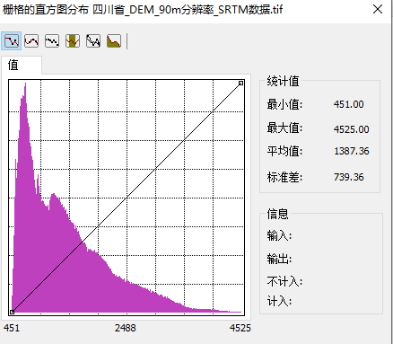
According to the DEM value distribution histogram of Sichuan Province, I made the following comparisons:
//Range comparison
//0-8000m
var palette_rainbow1 = palettes.kovesi.rainbow_bgyr_35_85_c72[7];
Map.addLayer(elevation, {min:0, max:8000, palette: palette_rainbow1},  'palette_rainbow1');
//Maximum and minimum
var palette_rainbow2 = palettes.kovesi.rainbow_bgyr_35_85_c72[7];
Map.addLayer(elevation, {min:188, max:7556, palette: palette_rainbow2},  'palette_rainbow2');
//Maximum and minimum values of horizontal axis of histogram
var palette_rainbow3 = palettes.kovesi.rainbow_bgyr_35_85_c72[7];
Map.addLayer(elevation, {min:451, max:4525, palette: palette_rainbow3},  'palette_rainbow3');
//The minimum value of the horizontal axis of the histogram is 6000
var palette_rainbow4 = palettes.kovesi.rainbow_bgyr_35_85_c72[7];
Map.addLayer(elevation, {min:451, max:6000, palette: palette_rainbow4},  'palette_rainbow4');
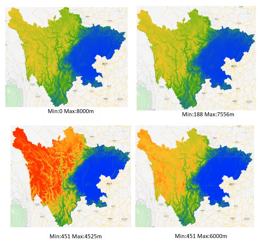
How to select the appropriate range of color palette is also an important factor in the elegant rendering of DEM.
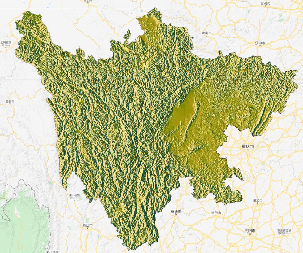
(3) Mountain shadow;
After selecting a better DEM data source, palette and value range, we can add mountain shadow to enhance the display effect of DEM. Function EE Terrain. Hillshade (input, azimuth, elevation) is the operator that generates mountain shadow. Input is DEM, azimuth is azimuth and elevation is altitude.
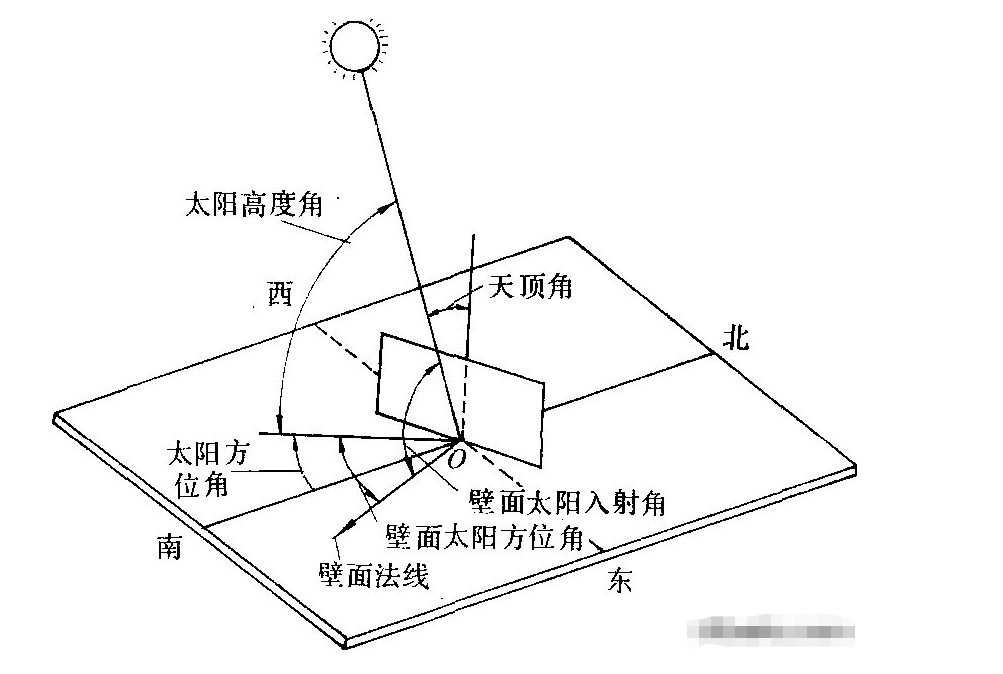
The azimuth refers to the angular direction of the sun. It is measured clockwise in the range of 0 to 360 degrees with north as the reference direction. The azimuth of 90 º is East. Height refers to the angle or slope of the lighting source above the horizon. The height is in degrees and ranges from 0 (on the horizon) to 90 (on the head). It should be noted that the value range of hillshade is 0-255
//Mountain shadow
var palette_hillshade = palettes.crameri.bamako[10,25,50];
var exaggeration = 20;
var hillshade = ee.Terrain.hillshade(elevation.multiply(exaggeration),270,45);
Map.addLayer(hillshade, {min: 0, max: 255, palette: palette_hillshade},  'palette_hillshade');
azimuth
There are azimuth angles that affect the display effect of mountain shadow:
//Different azimuth
var palette_hillshade = palettes.crameri.bamako[10,25,50];
var exaggeration = 20;
var hillshade_45 = ee.Terrain.hillshade(elevation.multiply(exaggeration),45,15);
Map.addLayer(hillshade_45, {min: 0, max: 255, palette: palette_hillshade},  'palette_hillshade_45');
var hillshade_135 = ee.Terrain.hillshade(elevation.multiply(exaggeration),135,15);
Map.addLayer(hillshade_135, {min: 0, max: 255, palette: palette_hillshade},  'palette_hillshade_135');
var hillshade_225 = ee.Terrain.hillshade(elevation.multiply(exaggeration),225,15);
Map.addLayer(hillshade_225, {min: 0, max: 255, palette: palette_hillshade},  'palette_hillshade_225');
var hillshade_315 = ee.Terrain.hillshade(elevation.multiply(exaggeration),315,15);
Map.addLayer(hillshade_315, {min: 0, max: 255, palette: palette_hillshade},  'palette_hillshade_315');
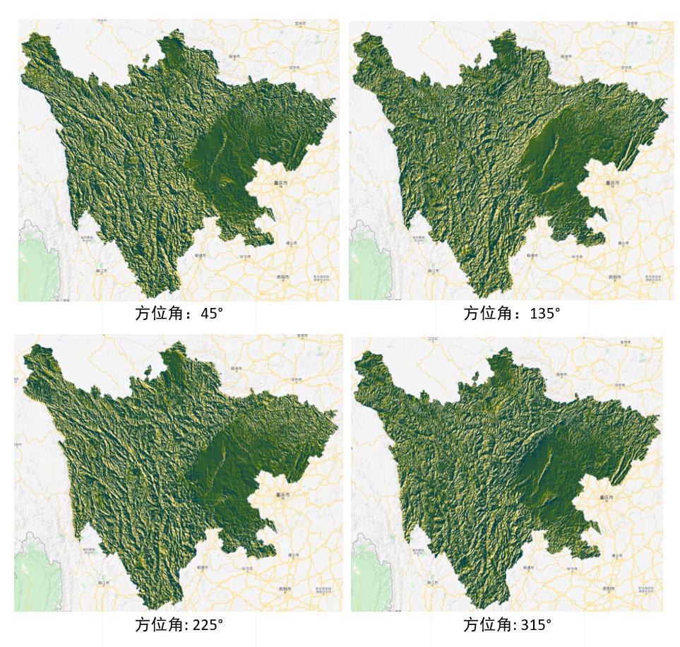
The default azimuth of GEE is 270 º, and the author can choose the appropriate azimuth according to his own needs.
Height angle
Different height angles will also affect the display effect of mountain shadow:
//Different height angles
var palette_hillshade = palettes.crameri.bamako[10,25,50];
var exaggeration = 20;
var hillshade_15 = ee.Terrain.hillshade(elevation.multiply(exaggeration),270,15);
Map.addLayer(hillshade_15, {min: 0, max: 255, palette: palette_hillshade},  'palette_hillshade_15');
var hillshade_30 = ee.Terrain.hillshade(elevation.multiply(exaggeration),270,30);
Map.addLayer(hillshade_30, {min: 0, max: 255, palette: palette_hillshade},  'palette_hillshade_30');
var hillshade_45 = ee.Terrain.hillshade(elevation.multiply(exaggeration),270,45);
Map.addLayer(hillshade_45, {min: 0, max: 255, palette: palette_hillshade},  'palette_hillshade_45');
var hillshade_60 = ee.Terrain.hillshade(elevation.multiply(exaggeration),270,60);
Map.addLayer(hillshade_60, {min: 0, max: 255, palette: palette_hillshade},  'palette_hillshade_60');
var hillshade_75 = ee.Terrain.hillshade(elevation.multiply(exaggeration),270,75);
Map.addLayer(hillshade_75, {min: 0, max: 255, palette: palette_hillshade},  'palette_hillshade_75');
var hillshade_90 = ee.Terrain.hillshade(elevation.multiply(exaggeration),270,90);
Map.addLayer(hillshade_90, {min: 0, max: 255, palette: palette_hillshade},  'palette_hillshade_90');
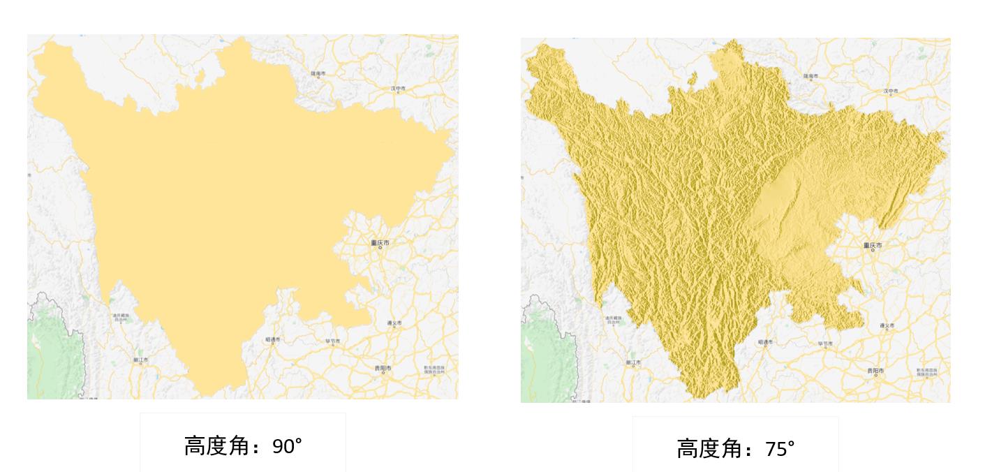
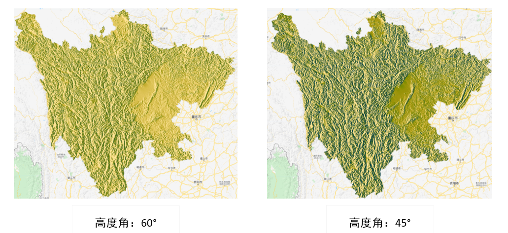

Generally speaking, the smaller the height angle, the stronger the mountain shadow effect. The default height angle in gee is 45 °.
Code link
https://code.earthengine.google.com/2e947952a68cb01eb63a247ec4424936
Write at the end
To sum up, we should use GEE to draw DEM gracefully:
Firstly, the data source must be selected, the DEM with high resolution can be selected for small research area, and the DEM with low resolution can be selected for large research area;
The second is to select the color palette. It is recommended to use the third-party library EE palettes, and then pay attention to the maximum value range of the color palette;
The second is to make mountain shadow, and pay attention to the selection of appropriate solar altitude and azimuth.
This article only provides a production idea. Due to the limited aesthetic level of the author, readers do not have to make topographic maps completely according to my color scheme. How to look good is how to do it.
reference resources
Clarmy squeaks How to draw cool three-dimensional topographic map with Python