1, Fundamentals of sorting algorithm
1. Algorithm classification
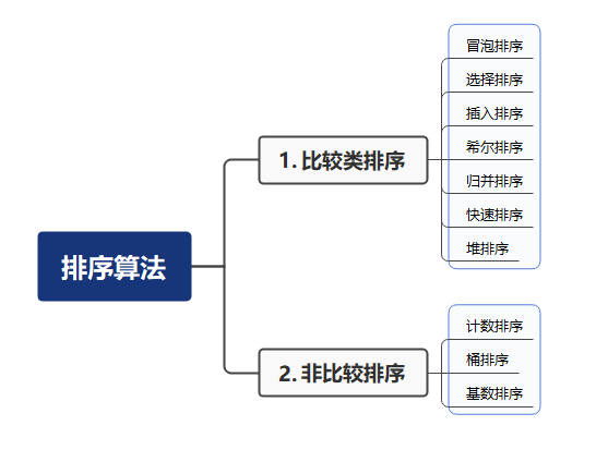
Common sorting algorithms can be divided into two categories:
Comparison sort: the relative order between elements is determined by comparison. Because its time complexity cannot exceed O(nlogn), it is also called nonlinear time comparison sort.
Non comparison sort: the relative order between elements is not determined by comparison. It can break through the lower bound of time based on comparison sort and run in linear time. Therefore, it is also called linear time non comparison sort.
2. Algorithm complexity
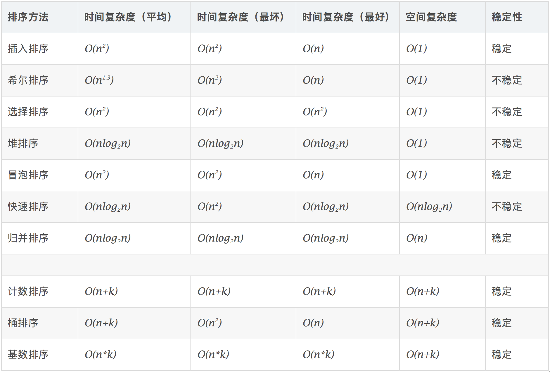
3. Basic concepts
Stability: if a was in front of b and a=b, a will still be in front of b after sorting.
Instability: if a was originally in front of b and a=b, a may appear after b after sorting.
Time complexity: the total number of operations on sorting data. Reflect the law of operation times when n changes.
Spatial complexity: refers to the measurement of the storage space required for the implementation of the algorithm in the computer. It is also a function of the data scale n.
2, Top ten sorting algorithms
1. Bubble Sort
1.1 algorithm description
Bubble sorting is a simple sorting algorithm. As the name suggests, bubble sorting is a comparison sorting algorithm that makes the larger (or smaller) numbers float to one end of the sequence like bubbles by comparing two numbers at a time.
The specific algorithm is described as follows:
- Compare adjacent elements. If the first one is bigger than the second, exchange them two;
- Do the same work for each pair of adjacent elements, from the first pair at the beginning to the last pair at the end, so that the last element should be the largest number;
- Repeat the above steps for all elements except the last one;
- Repeat steps 1 to 3 until the sorting is completed.
1.2 dynamic diagram demonstration
1.3 code implementation
void BubbleSort(vector<int> &arr) {
	int len = arr.size();
	for (int i = 0; i < len - 1; i++) {
		for (int j = 0; j < len - 1 - i; j++) {
			if (arr[j] > arr[j + 1]) {        // Pairwise comparison of adjacent elements
				int temp = arr[j + 1];        // Element exchange
				arr[j + 1] = arr[j];
				arr[j] = temp;
			}
		}
	}
}
2. Selection Sort
2.1 algorithm description
Selection sort is a simple and intuitive sorting algorithm. Its working principle: first, find the smallest (large) element in the unordered sequence and store it at the beginning of the sorted sequence, then continue to find the smallest (large) element from the remaining unordered elements, and then put it at the end of the sorted sequence. And so on until all elements are sorted.
The specific algorithm is described as follows:
- Initial state: the disordered area is R[1... n], and the ordered area is empty;
- At the beginning of the i-th sorting (i=1,2,3... n-1), the current ordered area and disordered area are R[1... i-1] and R(i... n) respectively. The sequence selects the record R[k] with the smallest keyword from the current unordered area and exchanges it with the first record r in the unordered area, so that R[1... I] and R[i+1... n) become a new ordered area with an increase in the number of records and a new unordered area with a decrease in the number of records respectively;
- At the end of n-1 trip, the array is ordered.
2.2 dynamic diagram demonstration

2.3 code implementation
void SelectionSort(vector<int> &arr) {
	int len = arr.size();
	int minIndex, temp;
	for (int i = 0; i < len - 1; i++) {
		minIndex = i;
		for (int j = i + 1; j < len; j++) {
			if (arr[j] < arr[minIndex]) {     // Find the smallest number
				minIndex = j;                 // Save the index of the smallest number
			}
		}
		temp = arr[i];
		arr[i] = arr[minIndex];
		arr[minIndex] = temp;
	}
}
3. Insertion Sort
3.1 algorithm description
The working principle of insertion sort is to build an ordered sequence. For unordered data, scan from back to front in the sorted sequence, find the corresponding position and insert.
The specific algorithm is described as follows:
- Starting from the first element, the element can be considered to have been sorted;
- Take out the next element and scan from back to front in the sorted element sequence;
- If the element (sorted) is larger than the new element, move the element to the next position;
- Repeat step 3 until the sorted element is found to be less than or equal to the position of the new element;
- After inserting the new element into this position; Repeat steps 2 to 5.
3.2 dynamic diagram demonstration

3.3 code implementation
void InsertionSort(vector<int> &arr) {
	int len = arr.size();
	int preIndex, current;
	for (int i = 1; i < len; i++) {
		preIndex = i - 1;
		current = arr[i];
		while (preIndex >= 0 && arr[preIndex] > current) {
			arr[preIndex + 1] = arr[preIndex];
			preIndex--;
		}
		arr[preIndex + 1] = current;
	}
}
4. Shell Sort
4.1 algorithm description
Hill sort is an improved version of simple insert sort. It differs from insert sorting in that it preferentially compares elements that are far away. Hill sort is also called reduced incremental sort.
Specific algorithm description:
- Select an incremental sequence t1, t2,..., tk, where ti > TJ, tk=1;
- Sort the sequence k times according to the number of incremental sequences k;
- For each sorting, the sequence to be sorted is divided into several subsequences with length m according to the corresponding increment ti, and each sub table is directly inserted and sorted. Only when the increment factor is 1, the whole sequence is treated as a table, and the table length is the length of the whole sequence.
4.2 dynamic diagram demonstration
4.3 code implementation
void ShellSort(vector<int> &arr) {
	int len = arr.size();
	for (int gap = len / 2; gap > 0; gap = gap / 2) {
		for (int i = gap; i < len; i++) {
			int j = i;
			int current = arr[i];
			while (j - gap >= 0 && current < arr[j - gap]) {
				arr[j] = arr[j - gap];
				j = j - gap;
			}
			arr[j] = current;
		}
	}
}
5. Merge Sort
5.1 algorithm description
Merge sort is an effective sort algorithm based on merge operation. The algorithm is a very typical application of Divide and Conquer. Merge the ordered subsequences to obtain a completely ordered sequence; That is, each subsequence is ordered first, and then the subsequence segments are ordered. If two ordered tables are merged into one, it is called 2-way merging.
Specific algorithm description:
- The input sequence with length n is divided into two subsequences with length n/2;
- Merge and sort the two subsequences respectively;
- Merge the two sorted subsequences into a final sorting sequence.
5.2 dynamic diagram demonstration
5.3 code implementation
void Merge(int arr[], int low, int mid, int high) {
	//low is the first element of the first ordered region, i points to the first element, and mid is the last element of the first ordered region
	int i = low, j = mid + 1, k = 0;  //mid+1 is the first element of the second ordered region, and j points to the first element
	int *temp = new int[high - low + 1]; //temp array temporarily stores the merged ordered sequence
	while (i <= mid&&j <= high) {
		if (arr[i] <= arr[j]) //The smaller ones are stored in temp first
			temp[k++] = arr[i++];
		else
			temp[k++] = arr[j++];
	}
	while (i <= mid)//If the first ordered area is still left after the comparison, it is directly copied to the t array
		temp[k++] = arr[i++];
	while (j <= high)//ditto
		temp[k++] = arr[j++];
	for (i = low, k = 0; i <= high; i++, k++)//Save the ordered data back to the range from low to high in the arr
		arr[i] = temp[k];
	delete[]temp;//To free memory, because it points to an array, you must use delete []
}

void MergeSort(int arr[], int low, int high) {
	if (low >= high) { return; } // The condition for terminating recursion. The length of the subsequence is 1
	int mid = low + (high - low) / 2;  // Gets the element in the middle of the sequence
	MergeSort(arr, low, mid);  // Recursion on the left half
	MergeSort(arr, mid + 1, high);  // Recursion to the right half
	Merge(arr, low, mid, high);  // merge
}
6. Quick Sort
6.1 algorithm description
Basic idea of quick sort: divide the records to be arranged into two independent parts through one-time sorting. If the keywords of one part of the records are smaller than those of the other part, the records of these two parts can be sorted separately to achieve the order of the whole sequence.
Specific algorithm description:
- Pick out an element from the sequence, which is called "pivot";
- Reorder the sequence. All elements smaller than the benchmark value are placed in front of the benchmark, and all elements larger than the benchmark value are placed behind the benchmark (the same number can be on either side). After the partition exits, the benchmark is in the middle of the sequence. This is called a partition operation;
- Recursively sorts subsequences that are smaller than the reference value element and subsequences that are larger than the reference value element.
6.2 dynamic diagram demonstration
6.3 code implementation
void Swap(vector<int> &arr, int i, int j) {
	int temp = arr[i];
	arr[i] = arr[j];
	arr[j] = temp;
}

int Partition(vector<int> &arr,int left,int right) {     // Partition operation
	int pivot = left,                      // Set reference value (pivot)
		index = pivot + 1;
	for (int i = index; i <= right; i++) {
		if (arr[i] < arr[pivot]) {
			Swap(arr, i, index);
			index++;
		}
	}
	Swap(arr, pivot, index - 1);
	return index - 1;
}

void QuickSort(vector<int> &arr, int left, int right) {
	int len = arr.size();
	int partitionIndex;

	if (left < right) {
		partitionIndex = Partition(arr, left, right);
		QuickSort(arr, left, partitionIndex - 1);
		QuickSort(arr, partitionIndex + 1, right);
	}
}
7. Heap Sort
7.1 algorithm description
Heap sort refers to a sort algorithm designed by using the data structure of heap. Heap is a structure similar to a complete binary tree, and satisfies the nature of heap at the same time: that is, the key value or index of a child node is always less than (or greater than) its parent node. Heap sorting uses the construction of large top heap (or small top heap). At the end of each construction, take the value of the top of the heap, and the resulting sequence is an ordered sequence.
Specific algorithm description:
- Build the initial keyword sequence to be sorted (R1,R2,... Rn) into a large top heap, which is the initial unordered area;
- Exchange the top element R[1] with the last element R[n], and obtain a new disordered region (R1,R2,... Rn-1) and a new ordered region (Rn), and meet R[1,2... N-1] < = R[n];
- Since the new heap top R[1] may violate the nature of the heap after exchange, it is necessary to adjust the current unordered area (R1,R2,... Rn-1) to a new heap, and then exchange R[1] with the last element of the unordered area again to obtain a new unordered area (R1,R2,... Rn-2) and a new ordered area (Rn-1,Rn). Repeat this process until the number of elements in the ordered area is n-1, and the whole sorting process is completed.
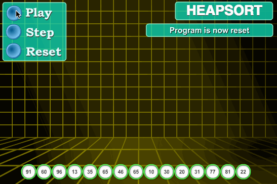
7.2 dynamic diagram demonstration
7.3 code implementation
void Adjust(int arr[], int len, int index)
{
	int left = 2 * index + 1;
	int right = 2 * index + 2;
	int maxIdx = index;
	if (left<len && arr[left] > arr[maxIdx]) maxIdx = left;
	if (right<len && arr[right] > arr[maxIdx]) maxIdx = right;  // maxIdx is the subscript of the largest of the three numbers
	if (maxIdx != index)                 // If the value of maxIdx is updated
	{
		swap(arr[maxIdx], arr[index]);
		Adjust(arr, len, maxIdx);       // Recursively adjust other parts that do not meet the nature of the heap
	}

}
void HeapSort(int arr[], int size)
{
	for (int i = size / 2 - 1; i >= 0; i--)  // Heap adjustment for each non leaf node (starting from the last non leaf node)
	{
		Adjust(arr, size, i);
	}
	for (int i = size - 1; i >= 1; i--)
	{
		swap(arr[0], arr[i]);           // Places the current largest at the end of the array
		Adjust(arr, i, 0);              // Continue the heap sort of the unfinished part
	}
}
8. Counting Sort
8.1 algorithm description
Counting sort is not a sort algorithm based on comparison. Its core is to convert the input data values into keys and store them in the additional array space. As a sort with linear time complexity, count sort requires that the input data must be integers with a certain range.
Specific algorithm description:
- Find the largest and smallest elements in the array to be sorted;
- Count the number of occurrences of each element with value i in the array and store it in item i of array C;
- All counts are accumulated (starting from the first element in C, and each item is added to the previous item);
- Reverse fill the target array: put each element i in item C(i) of the new array, and subtract 1 from C(i) for each element.
8.2 dynamic diagram demonstration
8.3 code implementation
void CountingSort(vector<int> &arr,int maxValue) {
	vector<int> bucket(maxValue + 1,0);
	int	sortedIndex = 0;
	int arrLen = arr.size();
	int	bucketLen = maxValue + 1;

	for (int i = 0; i < arrLen; i++) {
		if (!bucket[arr[i]]) {
			bucket[arr[i]] = 0;
		}
		bucket[arr[i]]++;
	}

	for (int j = 0; j < bucketLen; j++) {
		while (bucket[j] > 0) {
			arr[sortedIndex++] = j;
			bucket[j]--;
		}
	}
}
9. Counting Sort
9.1 algorithm description
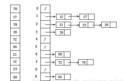
Bucket sorting is an upgraded version of counting sorting. It makes use of the mapping relationship of the function. The key to efficiency lies in the determination of the mapping function. Working principle of bucket sort: assuming that the input data is uniformly distributed, divide the data into a limited number of buckets, and then sort each bucket separately (it is possible to use another sorting algorithm or continue to use bucket sorting recursively).
Specific description of algorithm:
- Set a quantitative array as an empty bucket;
- Traverse the input data and put the data into the corresponding bucket one by one;
- Sort each bucket that is not empty;
- Splice the ordered data from a bucket that is not empty.
9.2 picture presentation
9.3 code implementation
//Bucket sorting
void BucketSort(vector<int> &arr,int bucketSize) {
	if (arr.size() == 0) {
		return ;
	}

	int i;
	int minValue = arr[0];
	int maxValue = arr[0];
	for (i = 1; i < arr.size(); i++) {
		if (arr[i] < minValue) {
			minValue = arr[i];                // Minimum value of input data
		}
		else if (arr[i] > maxValue) {
			maxValue = arr[i];                // Maximum value of input data
		}
	}

	// Initialization of bucket
	int DEFAULT_BUCKET_SIZE = 5;            // Set the default number of buckets to 5
	bucketSize = bucketSize || DEFAULT_BUCKET_SIZE;
	int bucketCount = (maxValue - minValue) / bucketSize + 1;
	vector<int> tmp;
	vector<vector<int>> buckets(bucketCount, tmp);


	// The mapping function is used to allocate the data to each bucket
	for (i = 0; i < arr.size(); i++) {
		buckets[(arr[i] - minValue) / bucketSize].push_back(arr[i]);
	}

	arr.resize(0);
	for (i = 0; i < buckets.size(); i++) {
		InsertionSort(buckets[i]);                      // Sort each bucket. Insert sort is used here
		for (int j = 0; j < buckets[i].size(); j++) {
			arr.push_back(buckets[i][j]);
		}
	}

}
10. Radix Sort
10.1 algorithm description
Cardinality sorting is to sort first according to the low order, and then collect; Then sort according to the high order, and then collect; And so on until the highest position. Sometimes some attributes have priority order. They are sorted by low priority first, and then by high priority. The final order is high priority, high priority first, high priority with the same low priority, high priority first.
Specific description of algorithm:
- Get the maximum number in the array and get the number of bits;
- arr is the original array, and each bit is taken from the lowest bit to form a radio array;
- Count and sort the radix (using the characteristics that count sorting is suitable for a small range of numbers);
10.2 dynamic diagram demonstration
10.3 code implementation
int Maxbit(vector<int> &data)
{
	int d = 1; //Save maximum number of digits
	int p = 10;
	for (int i = 0; i < data.size(); ++i)
	{
		while (data[i] >= p)
		{
			p *= 10;
			++d;
		}
	}
	return d;
}
void Radixsort(vector<int> &data) //Cardinality sort
{
	int d = Maxbit(data);
	vector<int> tmp(data.size(), 0);
	int count[10]; //Counter
	int i, j, k;
	int radix = 1;
	for (i = 1; i <= d; i++) //Sort d times
	{
		for (j = 0; j < 10; j++)
			count[j] = 0; //Clear the counter before each allocation
		for (j = 0; j < data.size(); j++)
		{
			k = (data[j] / radix) % 10; //Count the number of records in each bucket
			count[k]++;
		}
		for (j = 1; j < 10; j++)
			count[j] = count[j - 1] + count[j]; //Assign the positions in the tmp to each bucket in turn
		for (j = data.size() - 1; j >= 0; j--) //Collect all records in the bucket into tmp in turn
		{
			k = (data[j] / radix) % 10;
			tmp[count[k] - 1] = data[j];
			count[k]--;
		}
		for (j = 0; j < data.size(); j++) //Copy the contents of the temporary array to data
			data[j] = tmp[j];
		radix = radix * 10;
	}
}
3, References
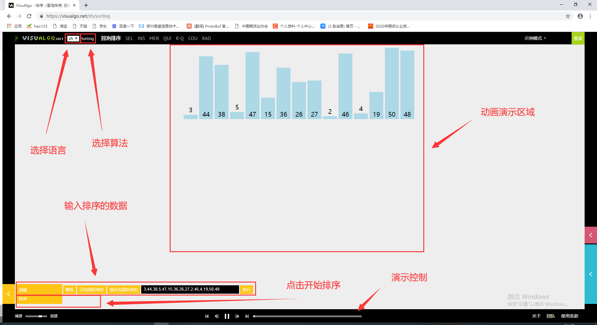
1. Dynamic diagram demonstration tool
The dynamic graph making of sorting algorithm is in VisuAlgo The website provides animation demonstrations of common sorting, search and other simple algorithms, which can help you learn vividly and concretely.
2. Sorting algorithm code (c + +)
All algorithm implementations involved in this article are packaged into a utils class with basic test code, Click to jump to the download address.
-----------------------------------------------------------------------------------------------------------------------------------------------------
❤️❤️❤️ Ten thousand words long article, if this article is helpful to you, please don't forget to like, pay attention to and collect three links with one button!!! ❤️❤️❤️
-----------------------------------------------------------------------------------------------------------------------------------------------------