1, Analysis purpose and data source

Analysis purpose:

• Understand the sales situation of the e-commerce platform from three aspects: products, customers and time zone;
• Identify important business standards to isolate customers and group customers into different value clusters to run targeted marketing strategies, reduce operating costs and improve revenue and efficiency;
• Put forward relevant suggestions on other aspects;

Data source:

This data is from kaggle, which records all transactions of an online retail store registered in the UK from January 12, 2010 to December 09, 2011. The company mainly sells various unique gifts, and its customers are mainly wholesalers.

Data link: https://www.kaggle.com/carrie1/ecommerce-data

2, Import and view dataset information

1. Import data

import warnings
import pandas as pd
import numpy as np
import matplotlib.pyplot as plt
import os

warnings.filterwarnings('ignore')  # Ignore alarm information
os.chdir(r"C:\Users\p\Desktop")
df = pd.read_csv('data.csv', encoding='ISO-8859-1', dtype={'CustomerID': str})
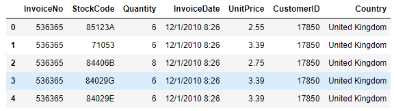
df.head()

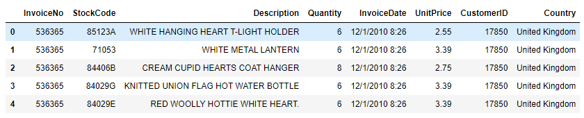
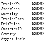
There are 8 field variables in the dataset:

2. View data information

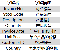
df.shape
df.info()

There are more than 540000 transaction records in the dataset. It can be seen from the dataset information that the Description and CustomerID fields are missing

3, Data preprocessing

1. Redundant and missing value handling

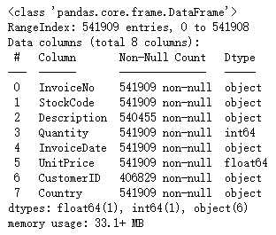
The missing rate of missing variables was calculated.

df.apply(lambda x :sum(x.isnull())/len(x),axis=0)

Here, since the Description has nothing to do with our analysis goal, it is removed. The CustomerID is the necessary data for subsequent sales analysis and customer classification. Considering that the missing rate of CustomerID is as high as 24.9%, deleting it will have a great impact on the accuracy of the analysis results, so it needs to be filled here.

df.drop(['Description'],axis=1,inplace=True)
df.head()
df['CustomerID'] = df['CustomerID'].fillna('Unknown')	

3. Duplicate value processing

To view the number of duplicate values in a dataset:

df.duplicated().sum()

Remove duplicates:

df = df.drop_duplicates()

3. Outlier handling

Descriptive statistics of data sets

df.describe()

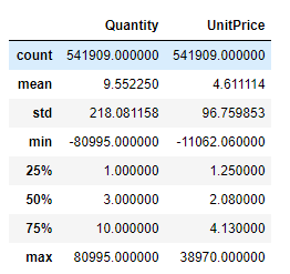
It can be seen from the description that both the sales quantity and the unit price of goods have negative values. If the sales quantity of goods is negative, it is speculated that it may be the return of goods. For the negative unit price of goods, this is meaningless and is judged as an abnormal value.

Take a closer look at the breakdown of commodity unit prices

df['UnitPrice'].groupby(df['UnitPrice']).count()
df[df["UnitPrice"]>0].count()

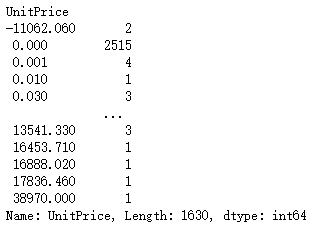
You can see that there are 2 with negative unit price, 2515 with zero unit price and 539392 with normal unit price. The unit price is zero, which can be understood as a gift.

Finally, don't forget to delete two abnormal records with negative unit price:

df = df[df['UnitPrice'] >= 0]

4. Variable processing

In order to more specifically analyze the sales of goods, the data set is divided into two parts: purchase and return. However, in order to avoid repeated variable operations, such as indicator disassembly and adding necessary fields, these two steps are advanced here.
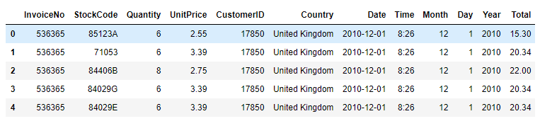
Split the date indicator and add the total sales indicator

df[["Date","Time"]]=df["InvoiceDate"].str.split(" ",expand=True)
df[["Month","Day","Year"]]=df["Date"].str.split("/",expand=True)
df.drop(['InvoiceDate'],axis=1,inplace=True)	# After splitting, the original InvoiceDate field can be deleted
df['Date'] = pd.to_datetime(df['Date']) 	#Convert Date to standard Date format
df["Total"]=df["Quantity"]*df["UnitPrice"]	# Add sales field
df.head()

First, check whether there is an exception that the purchase quantity of goods with an order is 0:

df[df["Quantity"] == 0]

The result shows that there is no abnormal situation with the purchase quantity of 0. Then, the data set is divided into two parts: commodity purchase information and return information:

df_buy = df[df["Quantity"] > 0]	# Purchase commodity data
df_return = df[df["Quantity"] < 0]	# Returned goods data

4, Data analysis

1. From the perspective of commodities

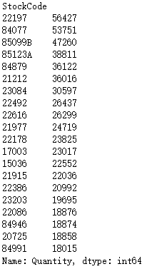
1.1 hot goods and goods with the most returns

quantity_sort=df["Quantity"].groupby(df["StockCode"]).sum().sort_values(ascending=False)
quantity_sort[:20]

Top 20 best selling products:

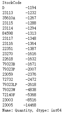
quantity_sort[-20:]

The top 20 commodities with the most returns are ranked, and the bottom is the one with the most returns, which decreases upward in turn:

1.2 what is the price distribution of goods and the sales volume of each price range?

df_unique_stock=df.drop_duplicates(["StockCode"])	# Count the types of goods
df_unique_stock['UnitPrice'].describe()	# Price description

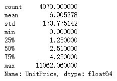
From the descriptive statistics, it can be seen that the average price of goods is 6.9 > the median price of goods is 2.51, which belongs to the right deviation distribution, indicating that most of the website sells low-priced goods, a small number of high-priced goods are expensive, a few high-priced goods increase the average value, and the standard deviation of commodity prices is large.

Now let's take a look at the specific price distribution of the goods on sale on the website:

# The unit price is grouped according to the mean and median
web_price_cut=pd.cut(df_unique_stock['UnitPrice'],bins=[0,1,2,3,4,5,6,7,10,15,20,25,30,50,100,10000]).value_counts().sort_index()
web_p_per=web_price_cut/web_price_cut.sum()
web_p_cumper=web_price_cut.cumsum()/web_price_cut.sum()
web_p_dis=pd.concat([web_p_per,web_p_cumper],axis=1)
web_p_dis
web_p_per=pd.DataFrame(web_p_per).reset_index()

# Drawing display
%matplotlib inline
plt.rcParams['font.sans-serif'] = ['SimHei']  # Used to display Chinese labels normally
plt.rcParams['axes.unicode_minus'] = False  # Used to display negative signs normally
plt.figure(figsize=(15,6))
x=web_p_per['index'].astype("str")
y=web_p_per['UnitPrice']
plt.bar(x,y)
web_p_cumper.plot(c='g',linewidth=2.0)
plt.xlabel('Price range',size=15)
plt.ylabel('percentage',size=15)
plt.legend(['Cumulative percentage of each price range','Proportion of each price range'],loc='upper left')
plt.show()

Output result:


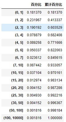
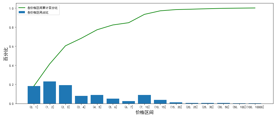
As can be seen from the chart, the number of commodity categories accounts for the highest proportion in the range of price (0,3), with a total of about 60%; commodities within 15 yuan account for 96.98%.

Let's take a look at the sales of goods at different prices:

cut=pd.cut(df['UnitPrice'],bins=[0,1,2,3,4,5,6,7,10,15,20,25,30,50,100,10000])
quan_price=df['Quantity'].groupby(cut).sum()
sale_p_per=quan_price/quan_price.sum()
sale_p_cumper=quan_price.cumsum()/quan_price.sum()
sale_p_dis=pd.concat([sale_p_per,sale_p_cumper],axis=1)
sale_p_dis.columns=['Proportion of sales volume','Cumulative proportion of sales']
sale_p_dis

# Drawing display
sale_p_per=pd.DataFrame(sale_p_per).reset_index()
plt.figure(figsize=(15,6))
x=sale_p_per['UnitPrice'].astype("str")
y=sale_p_per['Quantity']
plt.bar(x,y)
web_p_cumper.plot(c='g',linewidth=2.0)
plt.xlabel('Price range',size=15)
plt.ylabel('percentage',size=15)
plt.legend(['Cumulative proportion of sales volume in each price range','Proportion of sales volume in each price range'],loc='upper left')
plt.show()

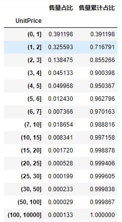
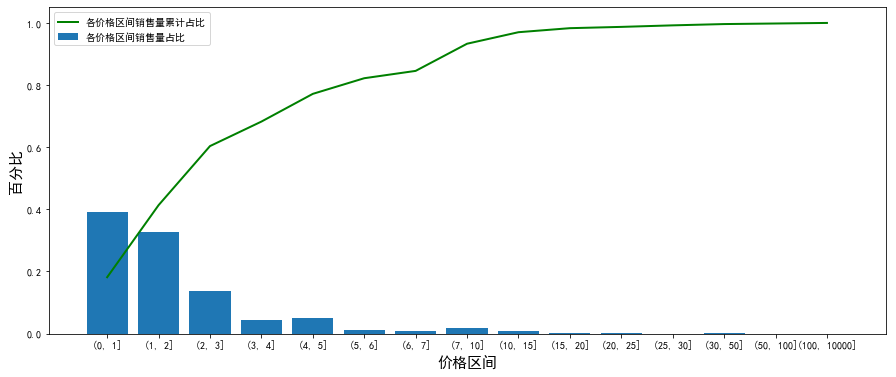
The chart shows that 85.5% of the sales are concentrated in goods with a price of less than 3 yuan, of which the proportion in the range of 0-1 is the highest, accounting for 39%, followed by the range of 1-2; The proportion of commodity sales within 15 yuan accounts for as high as 99.7%.

1.3 price distribution and quantity of returned goods

Group returned goods by different price ranges:

# Price slice of returned goods
cut1=pd.cut(df_return['UnitPrice'],bins=[0,1,2,3,4,5,6,7,10,15,20,25,30,50,100,10000])
return_group=df_return['Quantity'].groupby(cut1).sum()	# Price grouping for returned quantity
# Count the quantity proportion and cumulative quantity proportion of each price range of returned goods
per_cumper=pd.concat([return_group/return_group.sum(),return_group.cumsum()/return_group.sum()],axis=1)
per_cumper.columns=['Proportion of returned goods','Cumulative proportion of returned goods']
per_cumper

# Drawing display
return_per=pd.DataFrame(return_group/return_group.sum()).reset_index()
return_cumper=return_group.cumsum()/return_group.sum()
plt.figure(figsize=(15,6))
x=return_per['UnitPrice'].astype("str")
y=return_per['Quantity']
plt.bar(x,y)
return_cumper.plot(c='g',linewidth=2.0)
plt.xlabel('Price range',size=15)
plt.ylabel('percentage',size=15)
plt.legend(['Cumulative proportion of returned goods','Proportion of returned goods'],loc='upper left')
plt.show()

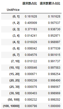
As can be seen from the figure, the price range of the most returned goods is 1 - 3, and the price is 3
The return of goods within accounted for 93.6%.
Comparison of returned goods at different prices and distribution of returned goods:

unique_stock=df_return.drop_duplicates('StockCode')	# Select all product categories
# Group all items by price
return_uni_group=pd.cut(unique_stock['UnitPrice'],bins=[0,1,2,3,4,5,6,7,10,15,20,25,30,50,100,10000]).value_counts().sort_index()

#Draw a picture to show the number of returned goods and the number of returned goods categories in different price ranges
plt.figure(figsize=(12,6))	
(return_group/return_group.sum()).plot(c='r')
(return_uni_group/return_uni_group.sum()).plot(c='b')
plt.xlabel('Price range',size=15)
plt.ylabel('percentage',size=15)
plt.legend(['Proportion of returned goods','Proportion of returned goods'])
plt.show()

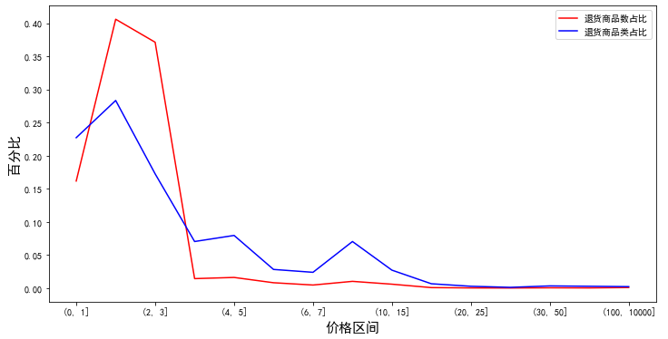
Compared with the price range 1-3 with the largest number of returned goods, the price range with the largest number of returned goods is 1-2. In addition, the price ranges 4-5 and 7-10 are also the ones with a large number of returned goods.

2. From the perspective of users

2.1 customers with the largest purchase amount and the highest purchase frequency

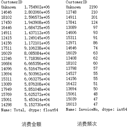
Calculate the top 20 customers with the largest consumption amount and the highest consumption frequency

# Consumption amount top20
customer_total=df_buy["Total"].groupby(df_buy["CustomerID"]).sum().sort_values(ascending=False)
customer_total[:20]

# Consumption frequency top20
customer_buy_freqency=df_buy.drop_duplicates(["InvoiceNo"])["InvoiceNo"].groupby(df_buy["CustomerID"]).count().sort_values(ascending=False)
customer_buy_freqency
customer_buy_freqency[:20]

2.2 distribution of commodity types of orders

Group by order, and check the type and quantity of goods purchased in each order:

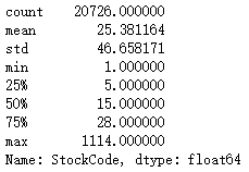
order_prodtype=df_buy['StockCode'].groupby(df_buy['InvoiceNo']).count().sort_values(ascending=False)
order_prodtype.describe()

Specific segmentation of order commodity types:

pd.cut(order_prodtype,bins=[0,25,50,100,200,300,500,1000,1200]).value_counts().sort_index()

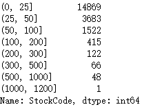
It can be seen from the description that there is a big gap in the number of goods in the order. By observing the average value and median value, it is found that the number of goods in the order is concentrated in about 25, while in half of the orders, the number of goods is less than 15, 75% of the orders are less than 28, and the number of goods in a very few orders is more than 100. Among these unreturned customers, Most of the order items are within 100.

Compare the returned goods:

# Group by order to view the description of the type and quantity of goods purchased in each return order
order_re_prodtype=df_return['StockCode'].groupby(df_return['InvoiceNo']).count().sort_values(ascending=False)
order_re_prodtype.describe()

# Segmented display
pd.cut(order_re_prodtype,bins=[0,5,10,20,30,40,50,100,120]).value_counts().sort_index()

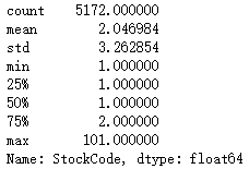
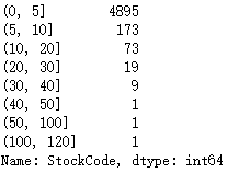
Compared with non return orders, most of the commodity types of return orders are within 10.

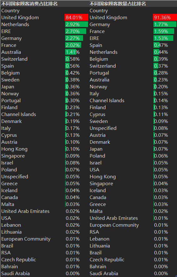
2.3 countries with the highest proportion of customer consumption, number of customers and average consumption of customers

# Proportion of customer consumption
country_total=df['Total'].groupby(df['Country']).sum().sort_values(ascending=False)
country_total_per=country_total/country_total.sum()
country_total_per

# Proportion of customers
country_customer=df['CustomerID'].groupby(df['Country']).count().sort_values(ascending=False)
country_customer_per=country_customer/country_customer.sum()
country_customer_per

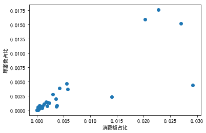
Draw a picture to view the distribution of countries by consumption and customers:

country_total_per.drop("United Kingdom",inplace=True)
country_customer_per.drop("United Kingdom",inplace=True)
plt.scatter(country_total_per.sort_index(),country_customer_per.sort_index())
plt.xlabel('Proportion of consumption')
plt.ylabel('Proportion of customers')

Let's look at the average consumption of customers in various countries:

df["Total"].groupby(df["Country"]).mean().sort_values(ascending=False)

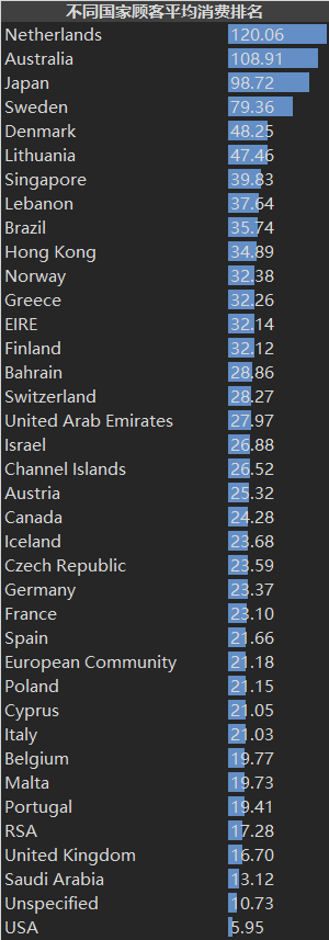
The e-commerce website has 91.36% of its customers and 84% of its sales from the UK. However, in terms of the average consumption of customers, the UK is only 16.7, ranking fourth from the bottom.
Excluding the extreme value of their own countries (the position in the red box in the figure), the countries with sales accounting for more than 1% include the Netherlands, Ireland, Germany, France and Australia; Countries with more than 1% of customers include Germany, France and Ireland; The countries with the highest average customer consumption are the Netherlands, Australia, Japan and Sweden, which can be the key targets for developing overseas markets.

2.4 RFM model customer segmentation

For e-businesses, they prefer to group customers into different clusters so that customized marketing activities can be carried out for each group, which will reduce customer acquisition costs and improve operating revenue. To do this, managers need to decide what are the important business criteria to isolate customers.
Smart operators know the importance of "know your customers". Operators must follow the paradigm shift from increasing click through to retention, loyalty and customer relationship building, rather than simply focusing on generating more clicks. Instead of analyzing the whole customer group, it is better to subdivide them into homogeneous groups, understand the characteristics of each group, and let them participate in relevant activities, rather than just subdivide the age or geography of customers. Therefore, RFM model is used here to subdivide customers to make precision marketing.

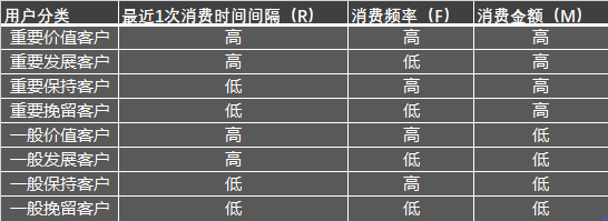
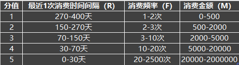
The meanings of indicators in RFM model are as follows:

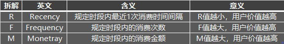
The consumption frequency and amount will affect the lifetime value of customers, while the last consumption interval will affect the retention rate, which will be an important indicator of participation (activity).

The customer segments scored by RFM are as follows:

Next, start modeling.

1) Calculate the user's last consumption interval - R value

# First ask the time of the user's last consumption
last_trans_date = df_buy.groupby('CustomerID')['Date'].max()
last_trans_date

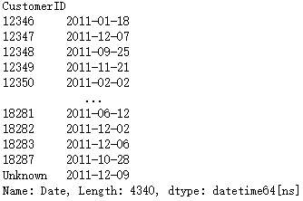
Here, the time span of the whole data is taken as the reference period, and the last day in the existing data is taken as the period boundary.

# The number of days between the user's last consumption and the reference time
R = (df_buy['Date'].max() - last_trans_date).dt.days
R

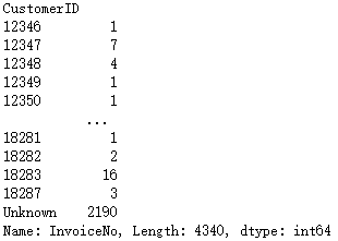
2) Calculate the user's consumption frequency - F value

Consumption frequency refers to the total consumption times of users in the specified period, which is the number of orders placed by users in the reference period.

# Number of orders placed by users - consumption frequency
F = df_buy.groupby('CustomerID')['InvoiceNo'].nunique()
F

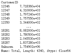
3) Calculate user's consumption amount - M value

The consumption amount here is the previously added sales variable, which can be summarized by user.

# Total consumption amount of users
M = df_buy.groupby('CustomerID')['Total'].sum()
M

4) R, F and M value scoring, customer value classification and summary

Draw the image distribution of R, F and M values:

import seaborn as sns
plt.figure(figsize=(6,18))
sns.set(style = 'darkgrid')

plt.subplot(2, 1, 2)
plt.hist(R,bins=30)
plt.xlabel('Days interval of last consumption')
plt.legend(['Number of users'],loc='upper right')
plt.subplot(2, 2, 1)
plt.hist(F,bins=30)
plt.xlabel('Consumption times')
plt.legend(['Number of users'],loc='upper right')
plt.subplot(2, 2, 2)
plt.hist(M,bins=30)
plt.xlabel('Consumption amount')
plt.legend(['Number of users'],loc='upper right')

plt.show()

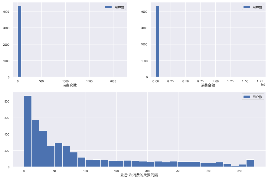
It can be seen from the figure that F and M indicators have serious abnormal values and great standard deviation. Check the descriptive statistics of each indicator:

R.describe()
F.describe()
M.describe()

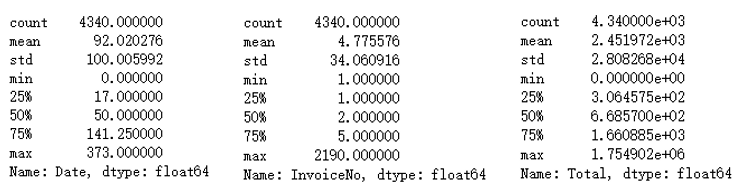
The above figure shows the descriptive statistical results of R, F and M values from left to right. Next, R, F and M are scored respectively on a 5-point scale according to the descriptive statistical results. Here, the scoring range threshold should be defined first. For businesses, the score of users should depend on the ranking of the index value of each user among the index values of all users, Of course, the scoring rules need to be set according to the specific business or seek the negotiation of the business department. Here is just a thought for reference.
Take the mean value in the statistical description as the medium score, then take the mean value from the minimum value to the mean value, and take the mean value from the mean value to the maximum value. Take this as the reference standard to formulate the scoring rule table
(or another idea can be used: rank r, F and M first, and then set the score limit for R, F and M by the percentile of interval threshold).

Grade R, F and M respectively:

# Split into 5 levels
R_bins = [0,30,70,150,270,400]
F_bins = [1,2,3,10,20,2500]
M_bins = [0,500,2000,5000,20000,2000000]

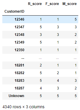
Slice R, F and M data and splice them into RFM scoring table:

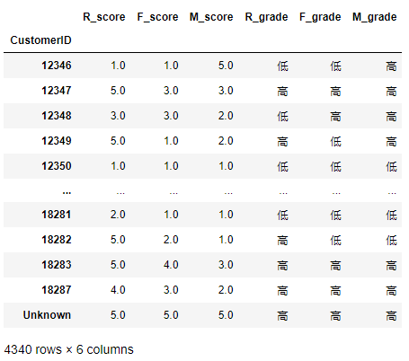
R_score = pd.cut(R,R_bins,labels=[5,4,3,2,1],right=False)
F_score = pd.cut(F,F_bins,labels=[1,2,3,4,5],right=False)
M_score = pd.cut(M,M_bins,labels=[1,2,3,4,5],right=False)
rfm = pd.concat([R_score,F_score,M_score],axis=1)
rfm.rename(columns={'Date':'R_score','InvoiceNo':'F_score','Total':'M_score'},inplace=True)
rfm

Change the types of R, F and M values and calculate their mean values:

for i in ['R_score','F_score','M_score']:
          rfm[i]=rfm[i].astype(float)
rfm.describe()

Score R, F and M values:

rfm['R_grade'] = np.where(rfm['R_score']>3.64,'high','low')
rfm['F_grade'] = np.where(rfm['F_score']>2.23,'high','low')
rfm['M_grade'] = np.where(rfm['M_score']>1.87,'high','low')
rfm

Value segmentation of users according to R, F and M ratings:

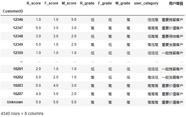
rfm['user_category']=rfm['R_grade'].str[:]+rfm['F_grade'].str[:]+rfm['M_grade'].str[:]
rfm['user_category'] =rfm['user_category'].str.strip()
 
def trans(x):
    if x=='Gao Gaogao':
        return 'Important value customers'
    elif x=='Height':
        return 'Key development customers'
    elif x=='Low high high':
        return 'Important to keep customers'
    elif x=='Low low high':
        return 'Important retention customers'
    elif x=='High and low':
        return 'General value customers'
    elif x=='High low':
        return 'General development customers'
    elif x=='Low height':
        return 'General customer retention'
    else:
        return 'General retention of customers'  
 
rfm['User level']=rfm['user_category'].apply(trans)
rfm

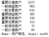
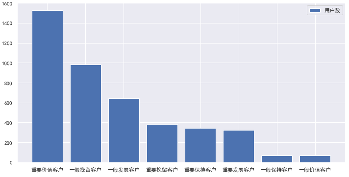
Summarize user segmentation results:

# Summary of various users
rfm['User level'].value_counts()

# Drawing display
plt.figure(figsize=(12,6))
plt.bar(rfm['User level'].value_counts().index,rfm['User level'].value_counts().values)
plt.legend(['Number of users'],loc='upper right')
plt.show()

3. Time dimension

3.1 quantity and amount of returned and unreturned goods in different months

In terms of return and non return, the number of orders and order amount are grouped by year and month.

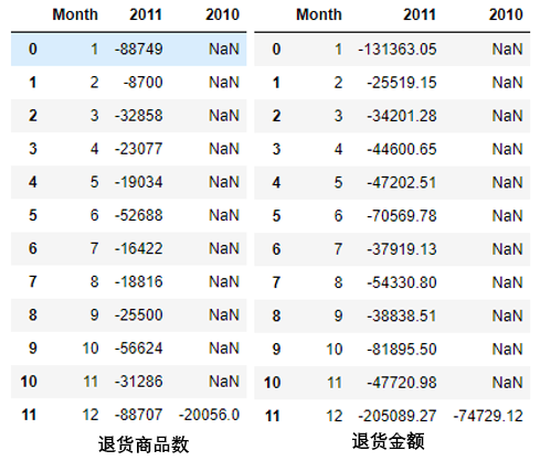
To view the quantity and amount of returned goods:

# Quantity of returned goods
df1 = df_return[df_return['Year']==2010]
df2 = df_return[df_return['Year']==2011]
temp1 = df2['Quantity'].groupby(df2['Month']).sum()
temp1 = pd.DataFrame(temp1).rename(columns={'Quantity':'2011'})
temp1['2010']=df1['Quantity'].groupby(df1['Month']).sum()
temp1 = temp1.reset_index()
# Return amount table
df3 = df_return[df_return['Year']==2010]
df4 = df_return[df_return['Year']==2011]
temp2 = df4['Total'].groupby(df4['Month']).sum()
temp2 = pd.DataFrame(temp2).rename(columns={'Total':'2011'})
temp2['2010']=df3['Total'].groupby(df3['Month']).sum()
temp2 = temp2.reset_index()

temp1.head()

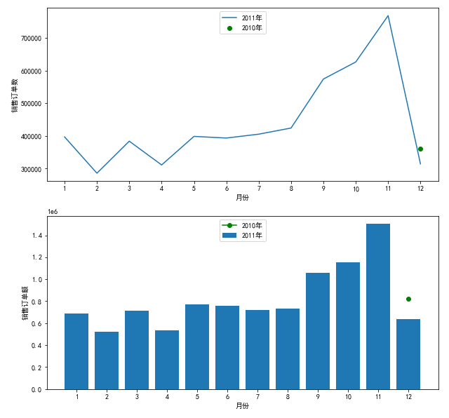
The bar chart shows the return amount and the breakdown of each order month

plt.figure(figsize=(10,10))
plt.subplot(2, 1, 1)
x1=temp1['month']
y1=np.abs(temp1['2011'])
y2=np.abs(temp1['2010'])
plt.scatter(x1,y2,c='g')
plt.plot(x1,y1)
plt.xlabel('month')
plt.ylabel('Number of returned orders')
plt.legend(['2011 year','2010 year'],loc='upper center')

plt.subplot(2, 1, 2)
x2=temp2['month']
y3=np.abs(temp2['2011'])
y4=np.abs(temp2['2010'])
plt.bar(x1,y3)
plt.plot(x1,y4,c='g',marker='o')
plt.xlabel('month')
plt.ylabel('Return order amount')
plt.legend(['2010 year','2011 year'],loc='upper center')
plt.show()

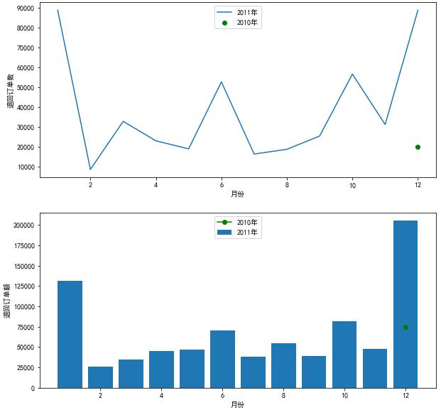
It can be seen from the figure that compared with other months, the return amount and return proportion in January and December are large. It is speculated that westerners may be in festivals such as Christmas at this time, and the shopping frequency is large. At the same time, the corresponding return frequency will be large. Similar to China's double 11, the increase of purchase will be accompanied by the increase of return.

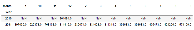
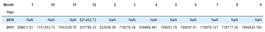
Similarly, draw the number and amount of unreturned goods:

3.2 sales amount, number of orders and average amount of orders in different months

Draw a picture to view the sales of different months:

df['Month']=df['Month'].astype('int')
df['Total'].groupby(df['Month']).sum().sort_index().plot()
plt.ylabel('sales volume')
plt.show()

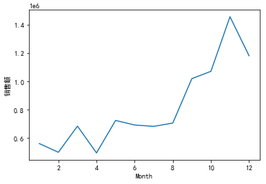
Sales showed an upward trend.

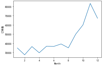
Draw a picture to view the number of orders in different months:

df['InvoiceNo'].groupby(df['Month']).count().sort_index().plot()
plt.ylabel('Number of orders')
plt.show()

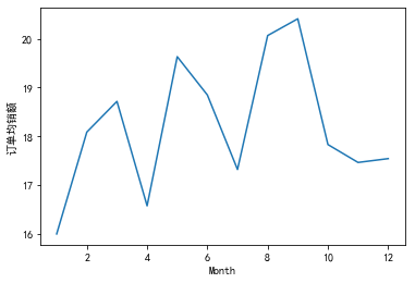
Then draw a picture to view the average sales of orders in different months:

df['Total'].groupby(df['Month']).mean().sort_index().plot()
plt.ylabel('Average sales of orders')
plt.show()

The total sales amount and the number of orders showed the same distribution. The total sales from January to December showed an upward trend with small fluctuations. The increase was the largest from August to November and reached the peak in November.
During the year, the average order amount fluctuated greatly, reaching a maximum in March, may and September respectively, of which September was the month with the largest average order amount in the whole year.

3.3 sales amount, number of orders and average amount of orders in different periods of the day

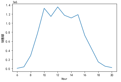
Draw a picture to show the sales amount at different times of the day:

df["Hour"]=df["Time"].str.split(":",expand=True)[0].astype("int")
df['Hour']=df['Hour'].astype('int')
df['Total'].groupby(df['Hour']).sum().sort_index().plot()
plt.ylabel('sales volume')
plt.show()

Similarly, draw the number of orders and average amount of orders in different periods of the day:


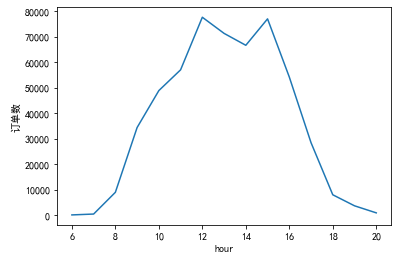
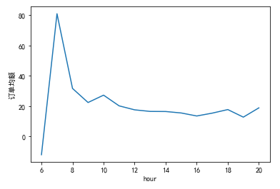
Orders with high total sales amount are mainly from 9:00 to 16:00, which are working hours, reaching the maximum value of the day at 10:00, 12:00 and 15:00 respectively. The largest number of orders is from 11 to 17, which is roughly the same as the distribution of sales amount. The time with the highest average order amount is 7 a.m., and there is little difference at other time points.

5, Conclusions and recommendations

1. Conclusion

• From the perspective of commodities, the situation of the website is as follows:
  1. What are the top 20 products that sell the most on the website and what are the top 20 products that return the most;
  2. The website mainly sells low-cost products wholesale, with 97% of the commodity unit price within 15. Among the commodities sold at low prices, the number of commodities in the 0 - 3 price range is the largest, accounting for about 60%;
  3. In terms of sales volume of goods, 95% of the sales volume of the website is concentrated within the unit price of 5, among which the goods in the price range of 0 - 2 are the best-selling, accounting for about 72%.
  4. The price of 94% of the returned goods on the website is lower than 5, and the goods with the price in the range of 1-3 account for the most, accounting for about 78%. For the types of returned goods, the number of returned goods is the largest in the price range of 1-2, followed by a large number of returned goods in the price range of 4-5 and 7-10.

• From the perspective of customers, the situation of the website is as follows:
  1. Who are the customers with the largest purchase amount and the most frequent purchases;
  2. Most of the successfully traded orders have less than 100 types of goods, of which 75% of the orders have less than 28 types of goods; The number of goods in the return order is mostly within 10;
  3. 91% of the customers of e-commerce websites come from China, and 84% of them have higher sales value; Abroad, the countries with high sales volume include the Netherlands, Ireland, Germany, France and Australia; Countries with a large number of customers include Germany, France and Ireland; Countries with high average customer consumption include the Netherlands, Australia, Japan and Sweden;
  4. 35% of the customers of the website are important value customers, 38% are general retention and development customers, 9%, 8% and 7% of the important retention, maintenance and development customers respectively, and the rest are other types of customers.

• From the perspective of time, the situation of the website is as follows:
  1) Since the purchase amount of customers and wholesalers should rise in the first month of the new year, the purchase amount of customers and wholesalers must rise in the first month of the new year; The average order amount reached the maximum in September; At the same time, because Westerners are in festivals such as Christmas, the return amount and return proportion in January and December are very large;
  2) The customers of the website are wholesalers rather than individuals, so they mainly place orders during working hours, of which 11-16 o'clock is the peak of orders.

2. Suggestion

• Commodities:
  1) Find out the advantages of hot goods and continue to maintain them. At the same time, pay attention to the out of stock vacancy management and regularly check whether the supply of hot goods is sufficient;
  2) Find your own main commodities and form your own advantageous commodity system, which can bring high sales and high gross profit. For example, for this e-commerce, the price of 95% of sales is less than 5, so it can be displayed at the lowest unit price on the commodity link page to attract customers' attention. You can do more promotional theme activities related to them on holidays.
  3) For the returned goods, the reasons for the most returned goods should be found out, and the products should be improved and optimized. The price of 94% of the returned goods on the website is lower than 5, and the price range with the most sales is exactly the price range with the most returns. Regardless of the time dimension, it shows that the home appliance manufacturer needs to take into account the quality of goods and the cultivation of added value of goods while looking for the reasons for customers' returns;

• Customers:
  1) For buyers with less than 10 types of goods in the order, collect more dimensional data and search for user portraits, classify such users and implement differentiated sales;
  2) Focus on the needs of domestic customers, and take the Netherlands, Ireland, Germany, France, Australia, Japan and Sweden as the key targets for developing overseas markets;
  3) Among classified users, important value customers are the best customers of the e-commerce. Their consumption habits have been maintained, with frequent consumption and the largest amount of consumption. To reward these customers, such as providing vip services to such customers, they can become early adopters of new products and contribute to brand promotion.
  4) For general customers who have not visited recently, organize relevant promotional activities to attract them back, investigate and find out what went wrong and avoid losing to competitors.
  5) For important development customers, we should find ways to increase their consumption frequency, increase the number of visits by providing induction support and special discounts, and take the initiative to establish relations with these customers to improve their repurchase rate;
  6) For important retention customers, they are loyal customers who often buy and spend a lot of money, but have not bought recently. Send them personalized reactivation activities and provide renewal and useful products to encourage them to buy again;
  7) Observe the main categories of goods purchased by customers who buy at high prices. And according to the purchase habits of these customers, do more promotional activities and exchange purchases related to them, so as to maintain their loyalty and recognition of the store;
  8) For other types of low value customers, we should also find out the possible reasons for no consumption, low consumption frequency and low consumption amount recently, and find ways to improve them.

• In terms of time:
  1) The number of orders has been increasing in one year, which indicates that the goods are basically recognized by customers. It is necessary to implement promotional activities during large holidays, such as November, to promote customers' purchase intention and increase their orders;
  2) It is expected that a large amount of goods, especially hot goods, will need to be prepared before the holidays. Sufficient manpower and resources should be arranged during the peak period of placing orders. At the same time, pay attention to observing and recording the detailed return information during this period, and communicate more with customers to find out the reasons for the return;