Elastic supervised learning enables you to train machine learning models based on the training examples you provide. Then, you can use your model to predict the new data. This article summarizes the end-to-end workflow of the training, evaluation, and deployment model. It outlines the steps required to identify and implement a solution using supervised learning. This article is a previous article“ Elastic search: data frame analysis using elastic machine learning ”A sequel to.
The workflow of supervised learning includes the following stages:
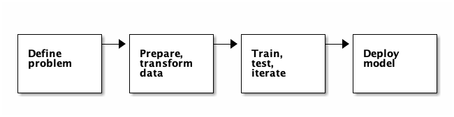
These are iterative phases, which means that after evaluating each step, you may need to make adjustments before proceeding further.
Definition problem
It's important to take a moment to think about where machine learning is most influential. Consider what type of data you have available and what value it has. The more you know about the data, the faster you can create machine learning models and generate useful insights. What patterns do you want to find in the data? What type of value do you want to predict: a category or a value? These answers can help you choose the type of analysis that is appropriate for your use case.
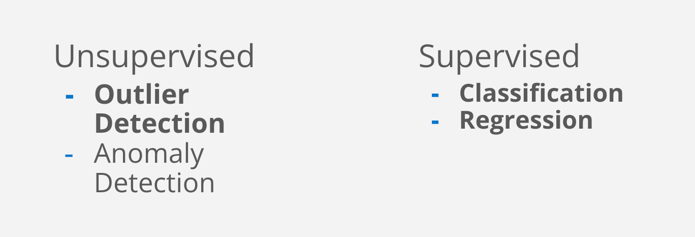
After identifying the problem, please consider which machine learning features are most likely to help you solve the problem. Supervised learning requires a data set containing known values that can train the model. Unsupervised learning - such as anomaly detection or anomaly detection - does not have this requirement.
Elastic Stack provides the following types of supervised learning:
- Region: predicts continuous values, such as the response time of Web requests. This variable can be changed continuously.
- Classification: predict discrete classification values, such as whether DNS requests come from malicious domains or benign domains (two classes). Or multiple classes, such as news categories: entertainment, sports, news, politics, etc.
Preparing and converting data
You have defined the problem and selected the appropriate analysis type. The next step is to generate high-quality data sets in Elasticsearch that are clearly related to your training objectives. If your data is not already in Elasticsearch, this is the stage when you develop the data pipeline. If you want to learn more about how to ingest data into Elasticsearch, see Ingestion node document.
Progression and classification are supervised machine learning techniques, so you must provide labeled data sets for training. This is often referred to as the "basic fact". The training process uses this information to identify the relationship between various features of the data and the predicted value. It also plays a vital role in model evaluation.
An important requirement is that the data set is large enough to train the model. For example, if you want to train a classification model to determine whether e-mail is spam, you need a tag dataset that contains enough data points from each possible category to train the model. What is "enough" depends on various factors, such as the complexity of the problem or the machine learning solution you choose. There are no exact numbers for each use case; Determining how much data is acceptable is a heuristic process that may involve iterative experiments.
Before training the model, consider preprocessing the data. In practice, the type of preprocessing depends on the nature of the data set. Preprocessing may include, but is not limited to, reducing redundancy, reducing deviation, applying standards and / or conventions, data normalization, etc.
Regression and Classificaiton require specially structured source data: two-dimensional table data structure. For this reason, you may need to transformation Use your data to create a data frame that can be used as a source for these types of data frame analysis. For a detailed introduction to data frame #, please refer to my previous article“ Elastic search: data frame analysis using elastic machine learning".
Training, testing, iteration
Once the data is ready and converted to the correct format, it's time to train the model. Training is an iterative process - it is evaluated after each iteration to understand the performance of the model.
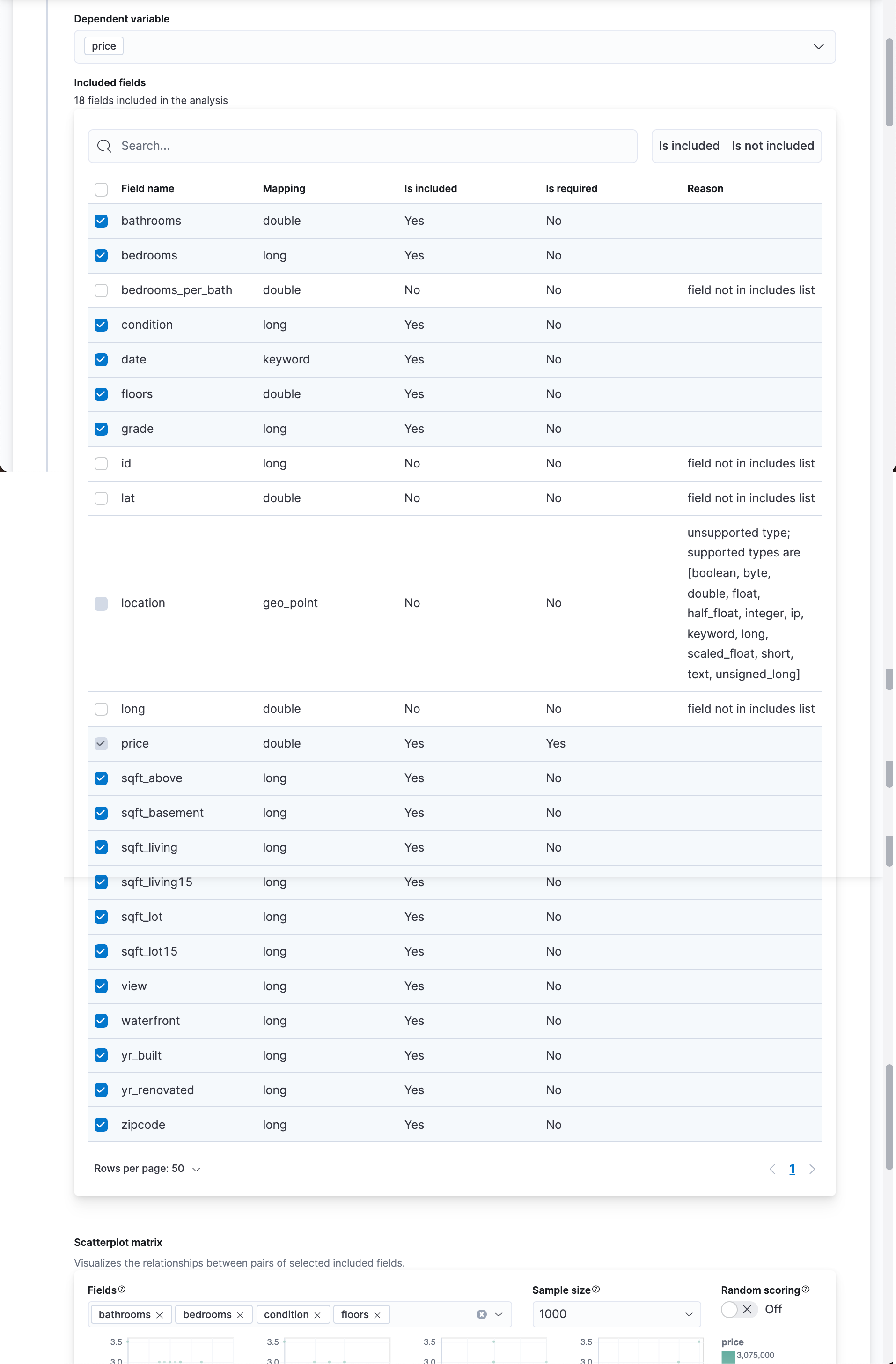
The first step is to define the features that will be used to train the model - the relevant fields in the dataset. By default, all fields of supported types are automatically included in region and classification. However, you can choose to exclude irrelevant fields from the process. This makes large data sets easier to manage and reduces the computational resources and time required for training.
Next, you must define how to split the data into training sets and test sets. The test set will not be used to train the model; It is used to evaluate the performance of the model. There is no optimal percentage for all use cases, depending on the amount of data and the time you have to train. For large datasets, you may want to start with a lower percentage of training to complete end-to-end iterations in a short time.
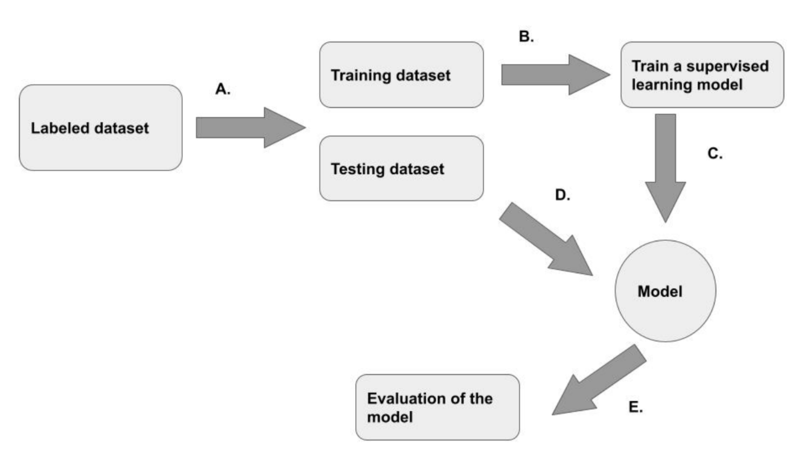
In the training process, the training data is input through the learning algorithm. The model predicts the value and compares it with the basic facts, and then fine tune the model to make the prediction more accurate.
For Classification, we can use the following figure to describe it:
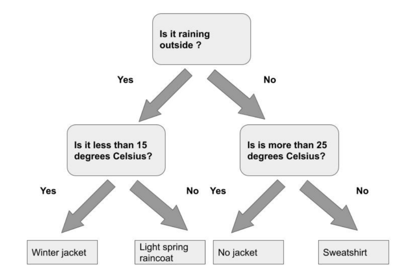
In the figure above, it shows that machine learning can help us determine the appropriate wearable clothes for a specific condition. As shown above, it contains different class es to choose from.
For Regression, we can use the following figure to describe it:
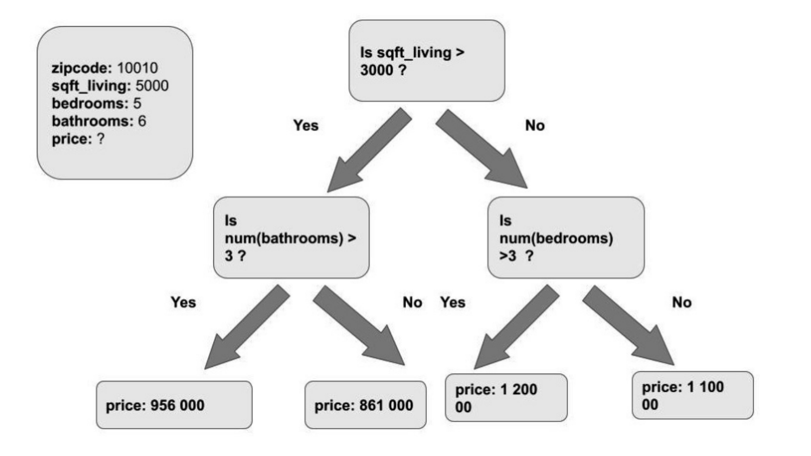
Unlike Classification, expression can predict continuously changing variable values. For the above figure, given certain conditions and using machine learning, we can predict the house price. For the above data model, see my previous article“ Elastic search: data frame analysis using elastic machine learning".
Deployment model
You have trained the model and are satisfied with the performance. The final step is to deploy the trained model and start using it on new data.
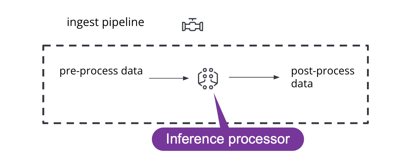
Elastic machine learning, called information, enables you to predict new data by using it as a processor in the intake pipeline, continuous conversion, or aggregation during search. When new data enters your ingestion pipeline or you run a search on the data using inference aggregation, the model is used to infer the data and predict it.
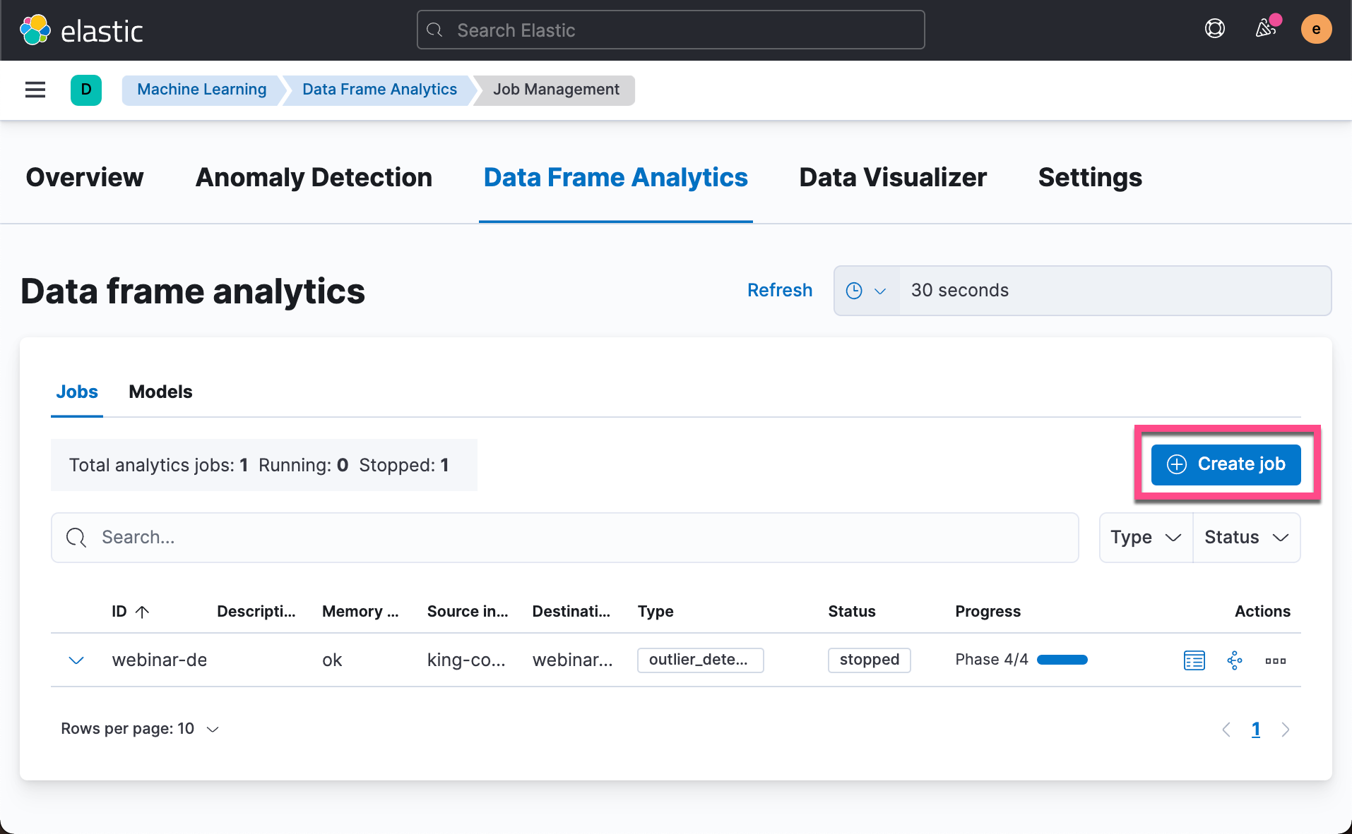
Supervised Learning demo
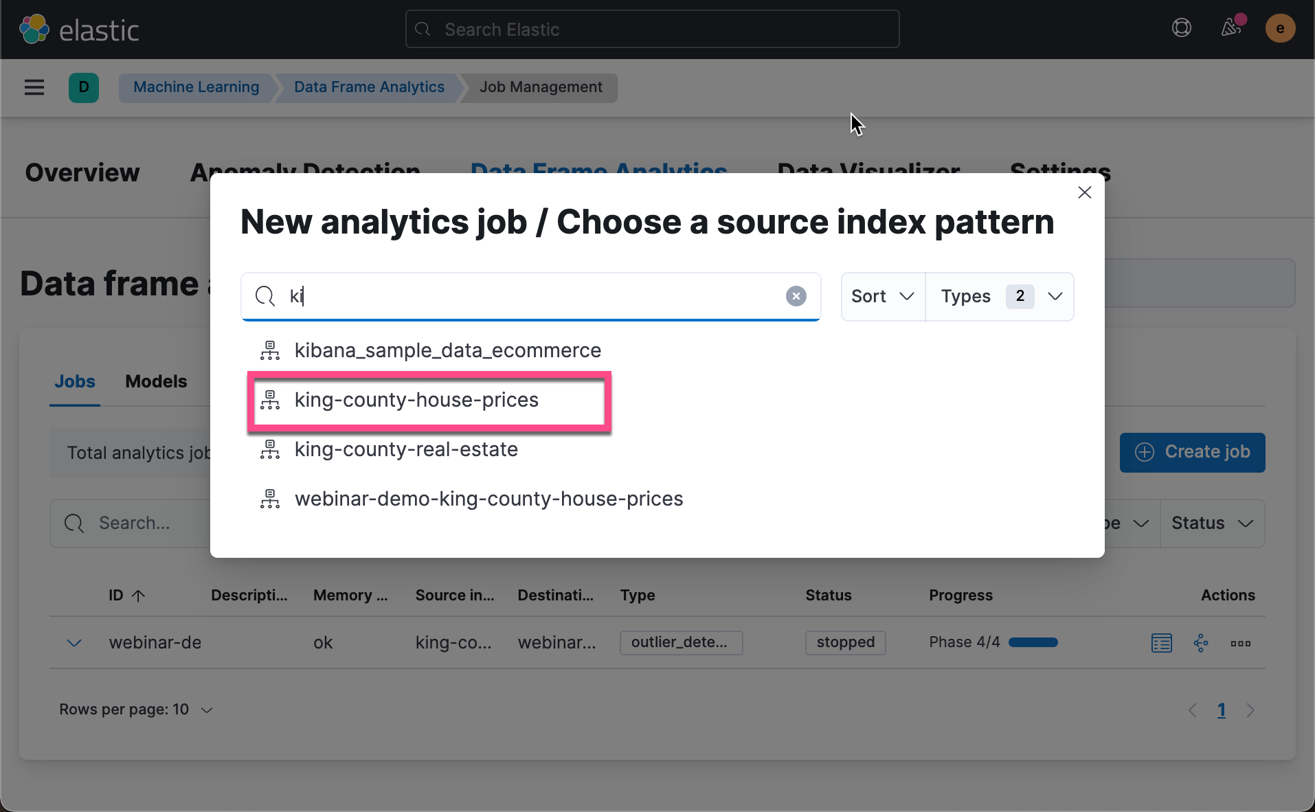
Let's prepare the data first. Let's go back to the previous article“ Elastic search: data frame analysis using elastic machine learning ”. In that article, we have successfully absorbed the house price information of King County in the United States. Let's continue the demonstration with that article.
Open Kibana:

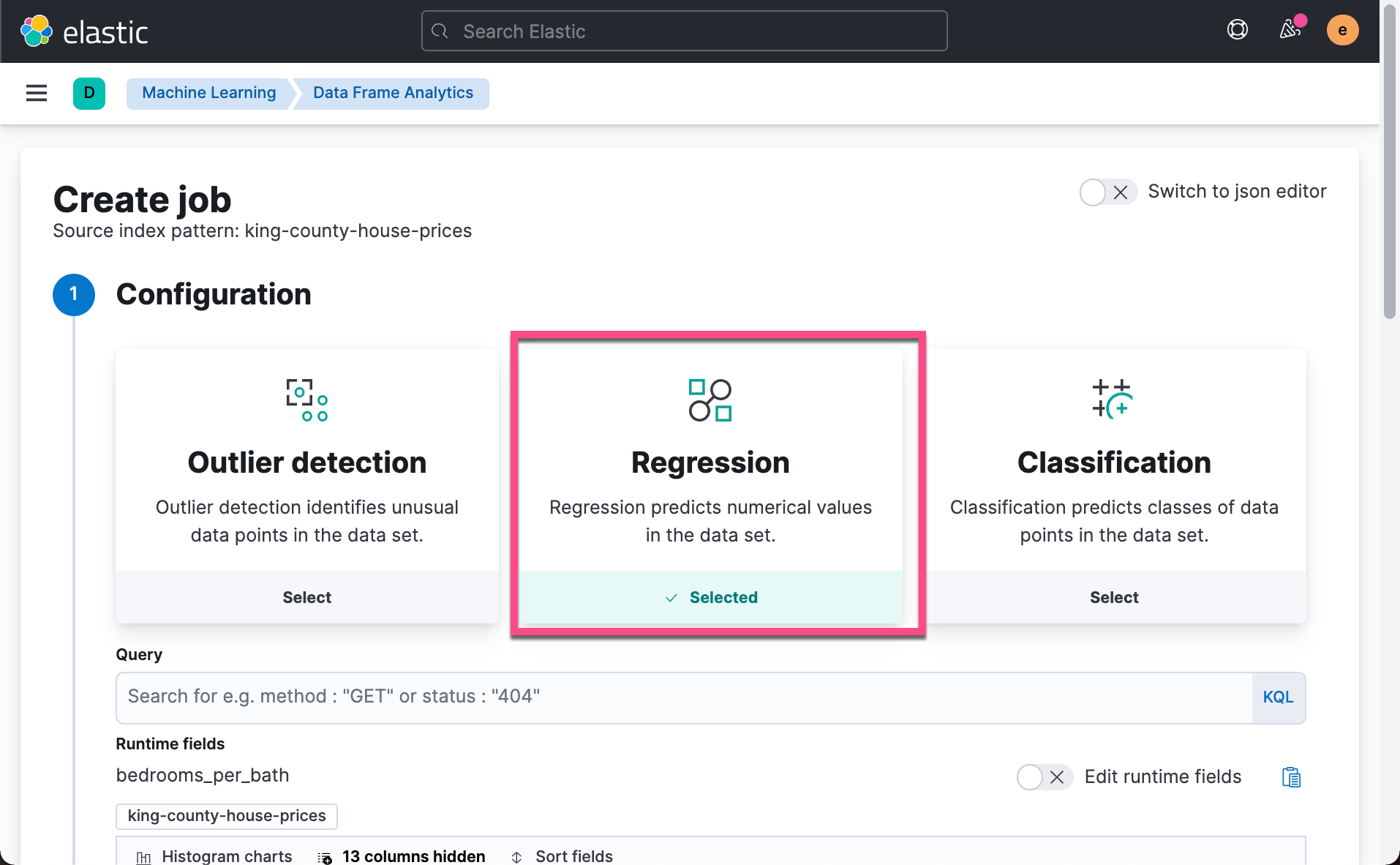
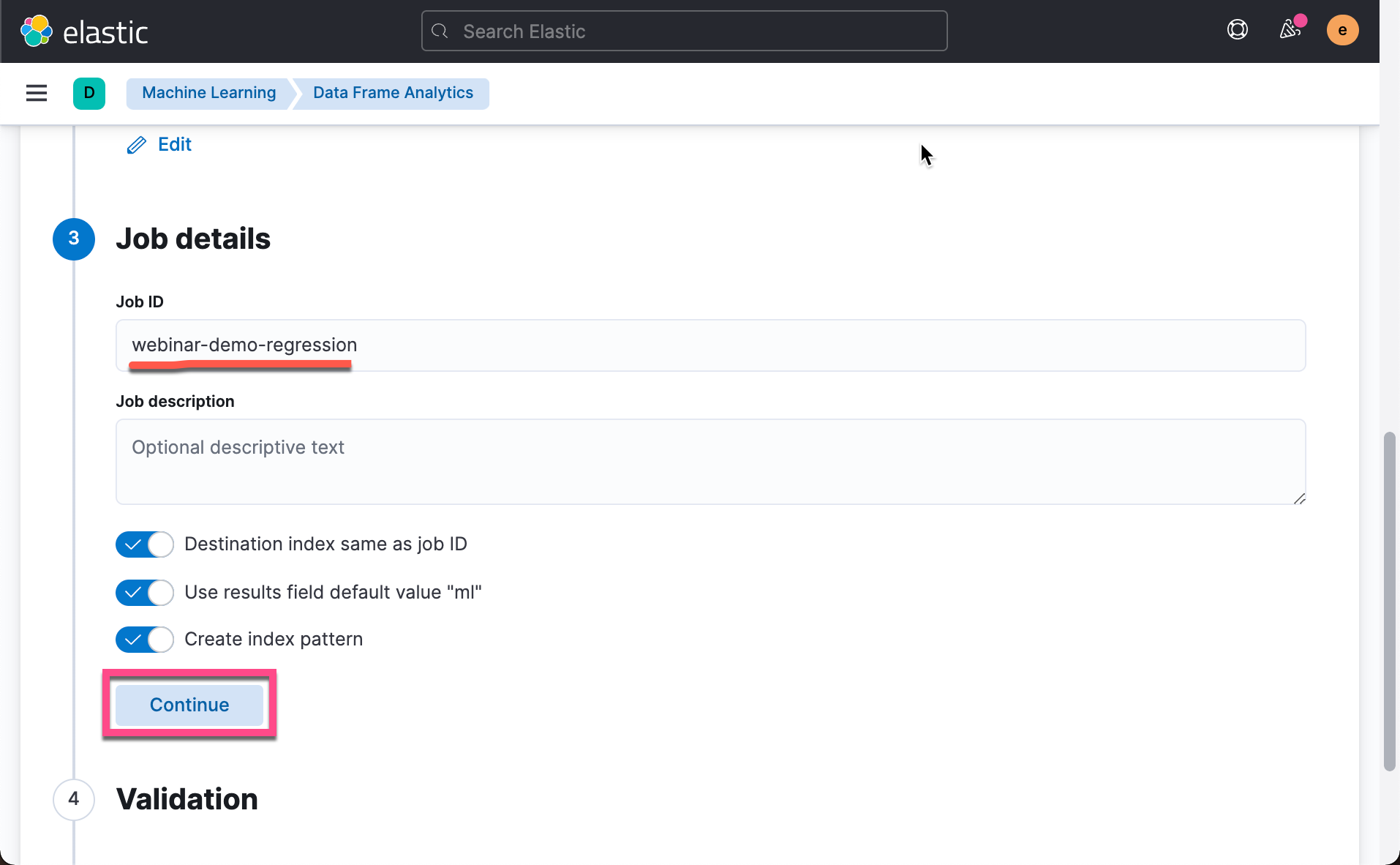
This time we choose Regression instead of Outlier detection.
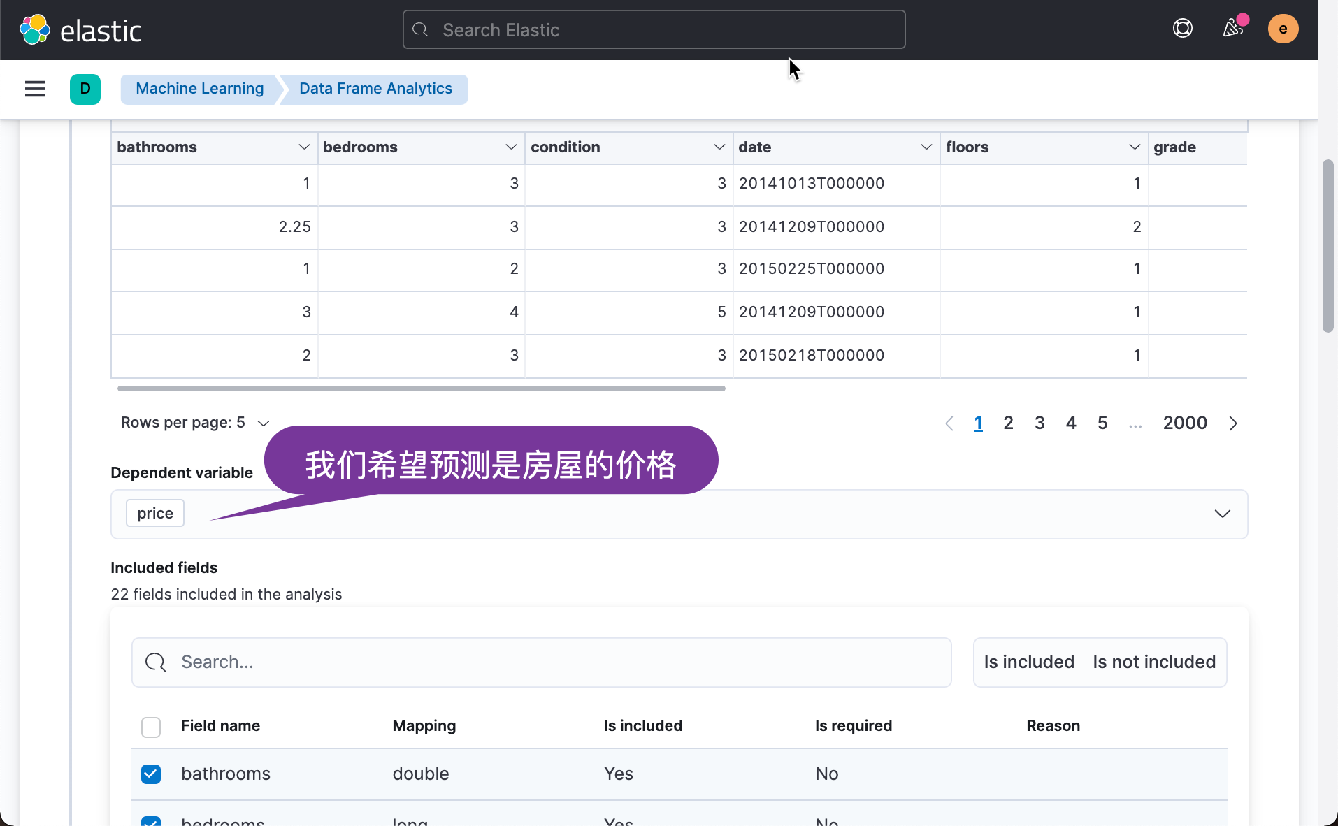
Next, we choose the parameters we are interested in to predict. For example, we can remove the id, longitude and latitude parameters:
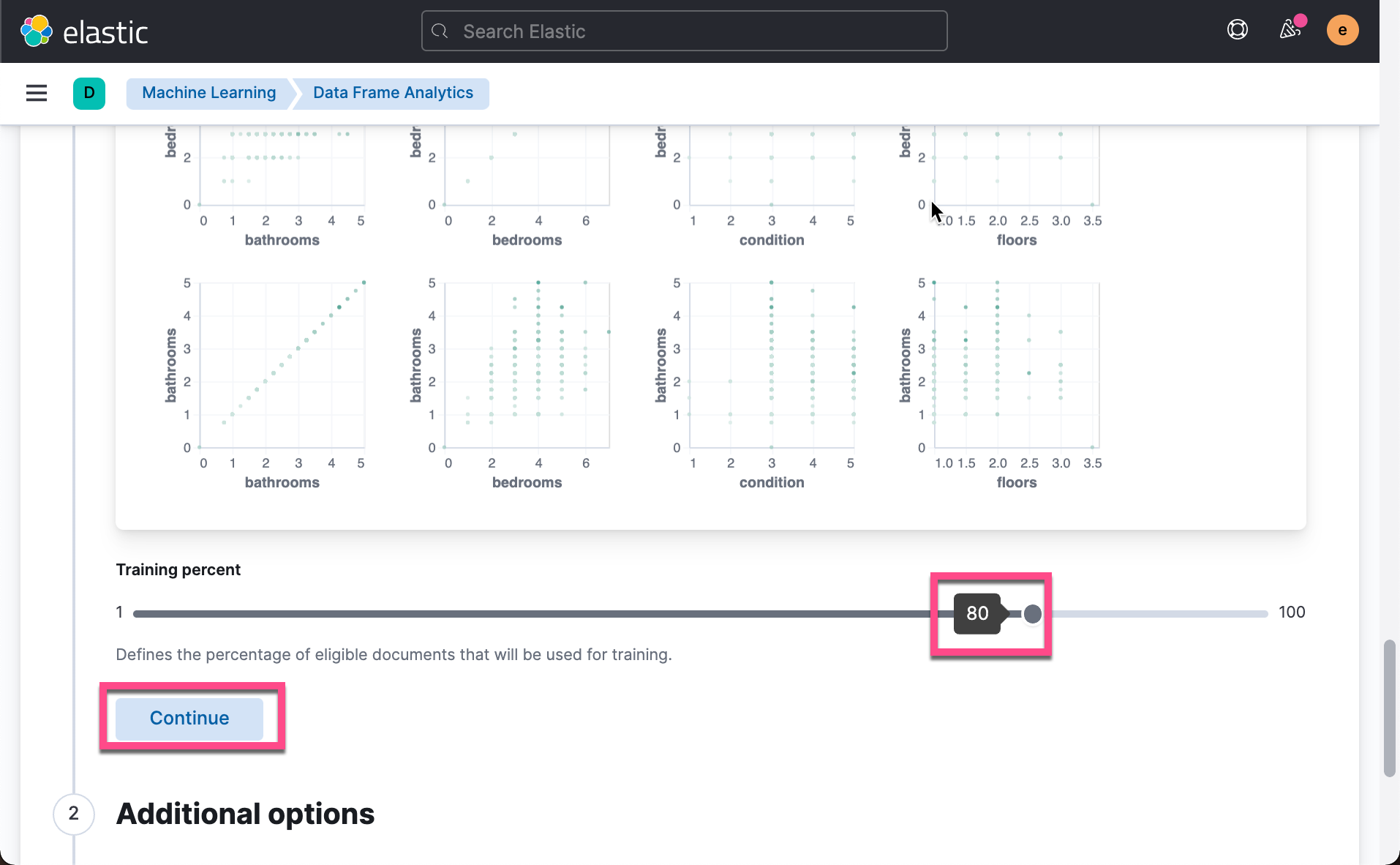
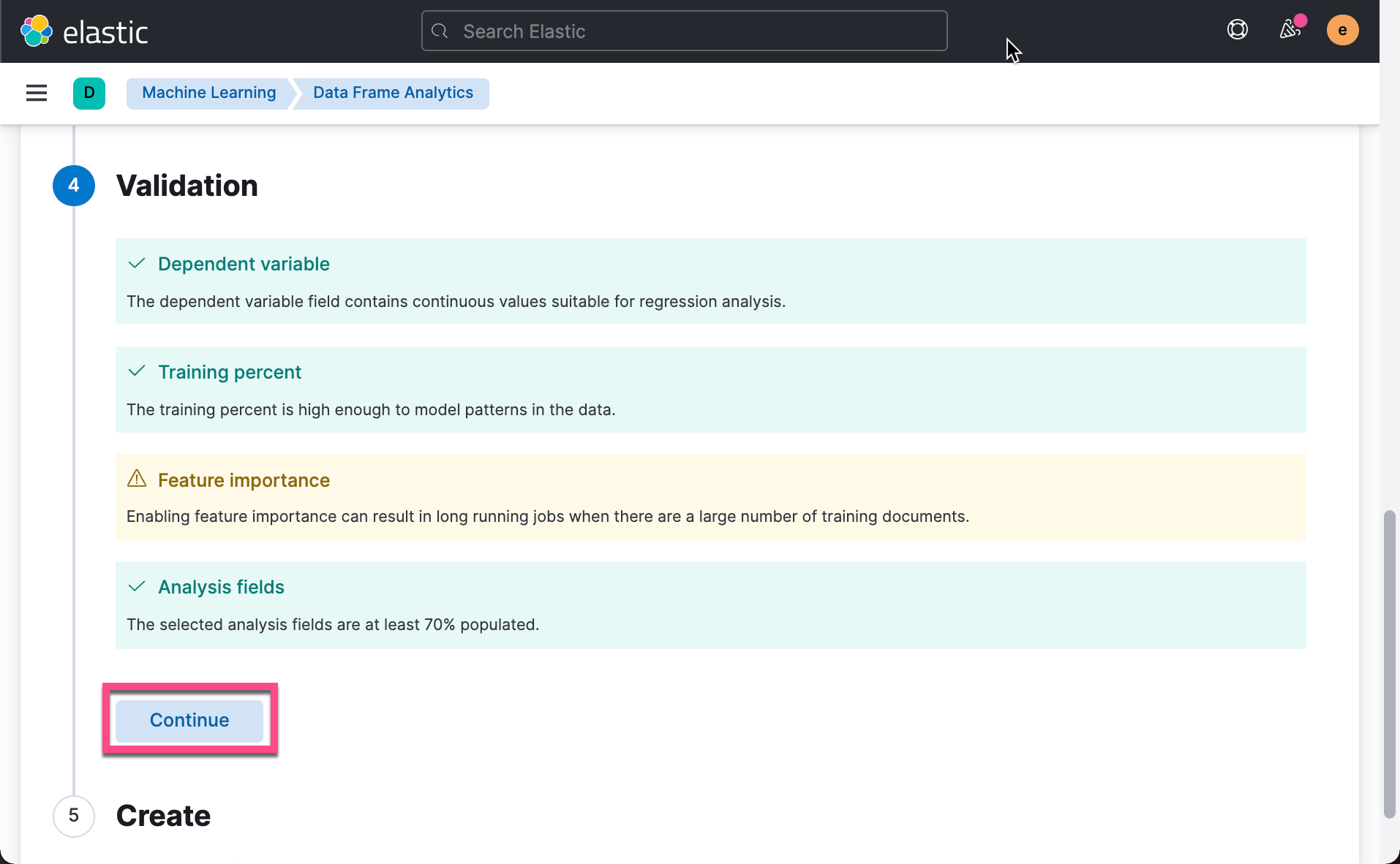
As we mentioned above, we need a certain data set for training, and we need to leave some data to test whether our model is correct. In the above, we can choose how much proportion of data to train. This ratio depends on how much data you have and how long it takes you to complete your training. If your data set is large, it is recommended that you use a small proportion for training and constantly correct it until you get the appropriate accuracy. In our case, our data set is not very large. We accept the default 80%. Click Continue above:
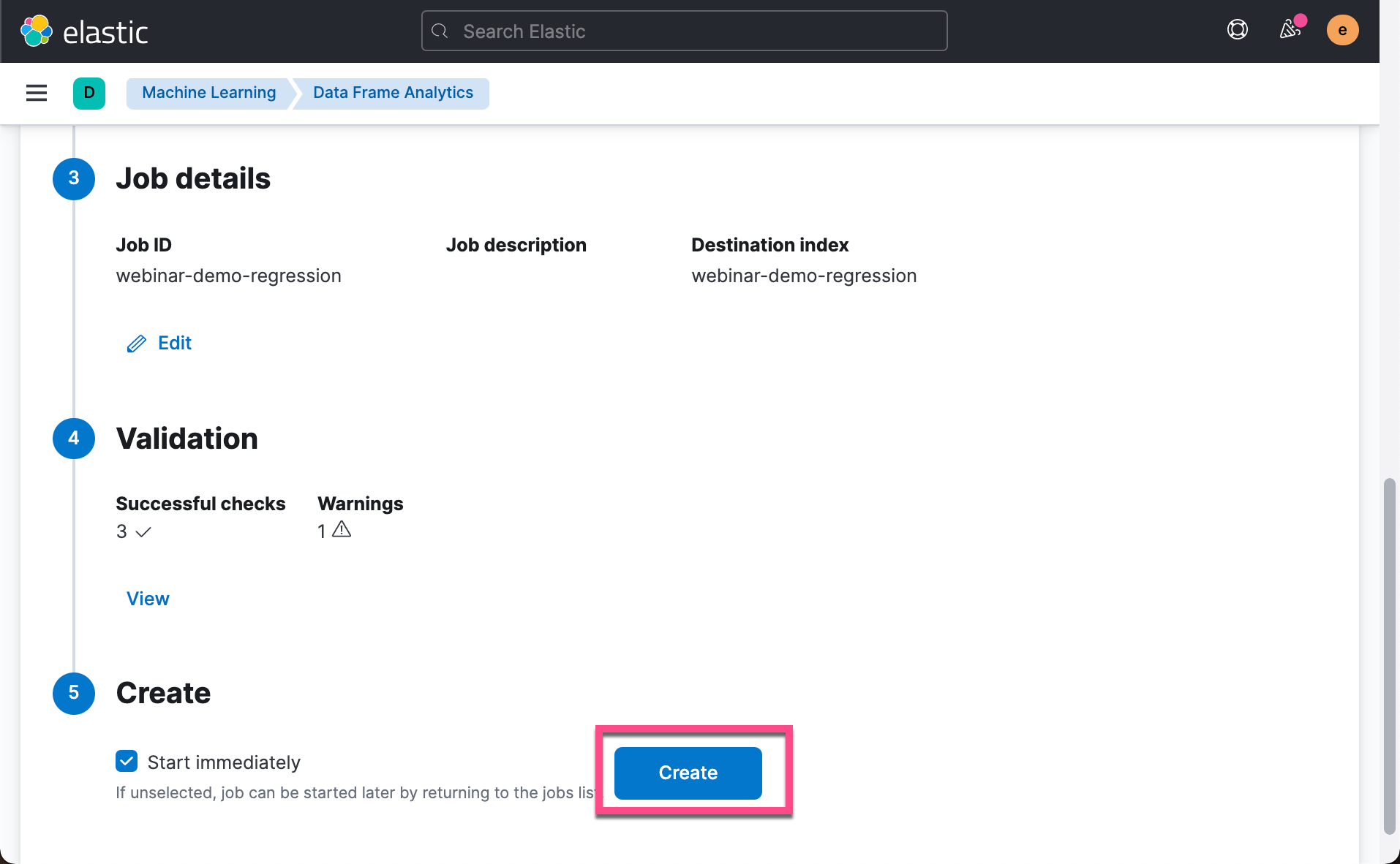
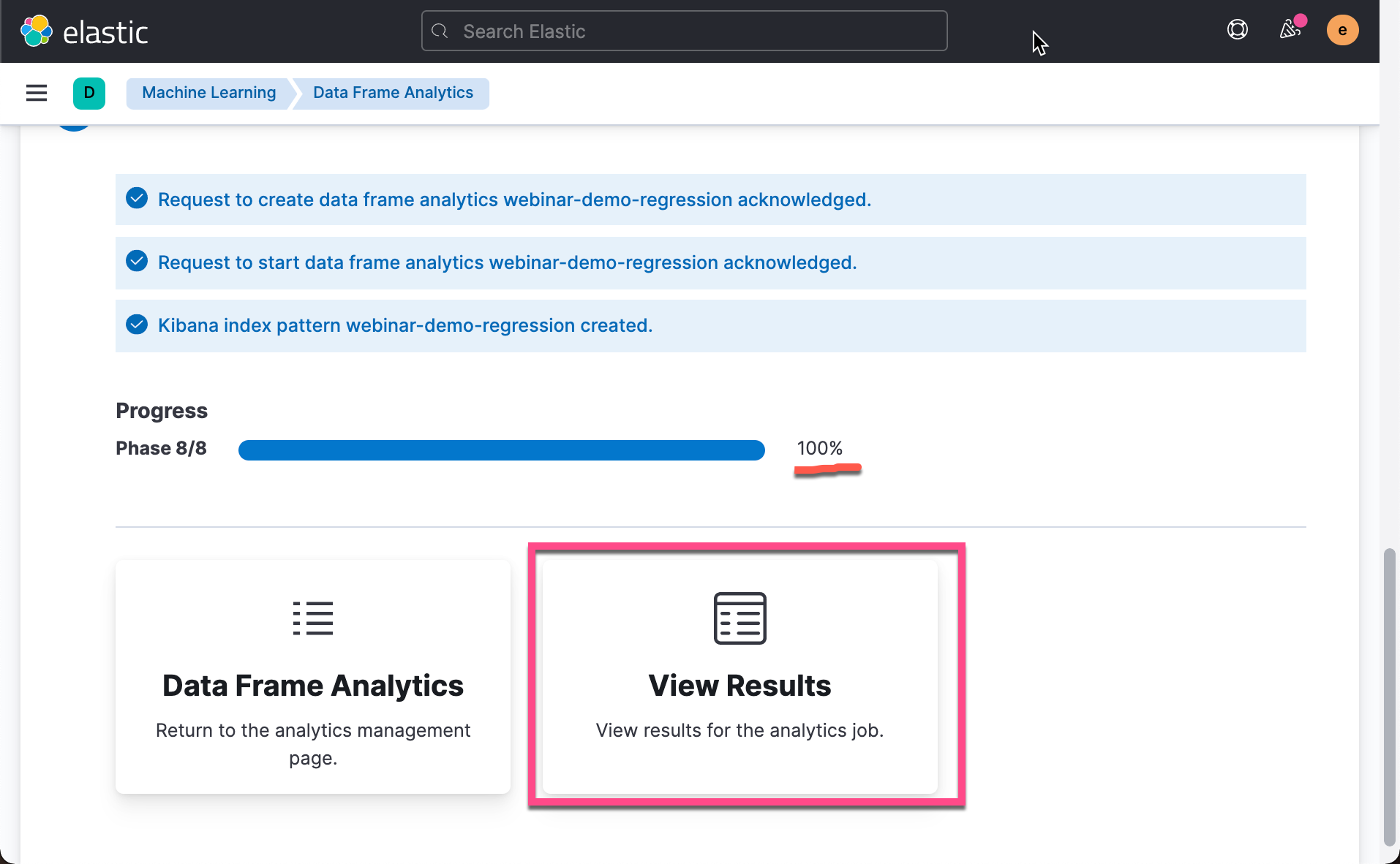
Click the Create button above. We need to wait a while before we can complete our machine learning training:
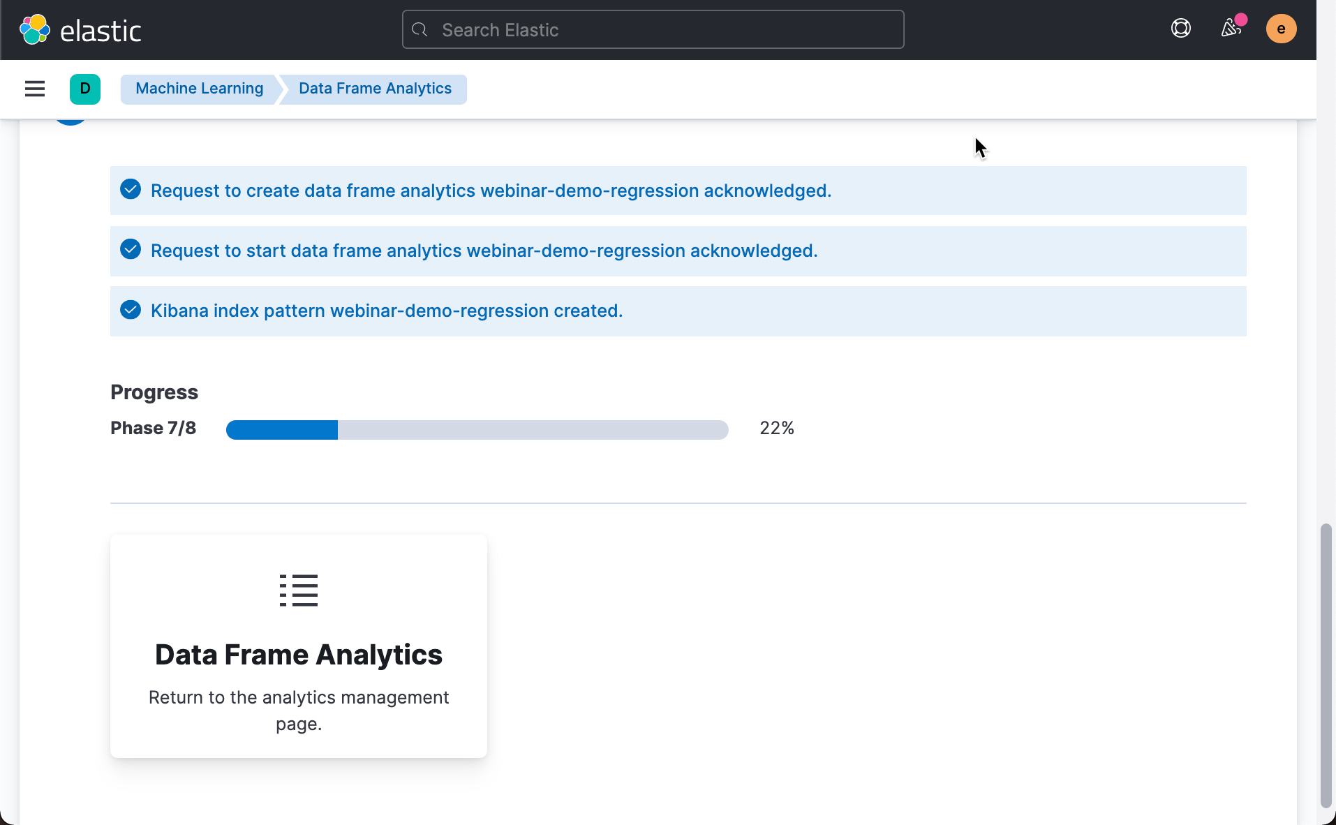
Depending on how many data sets you have, this time can be very long. In our case, this takes about 3-4 minutes:
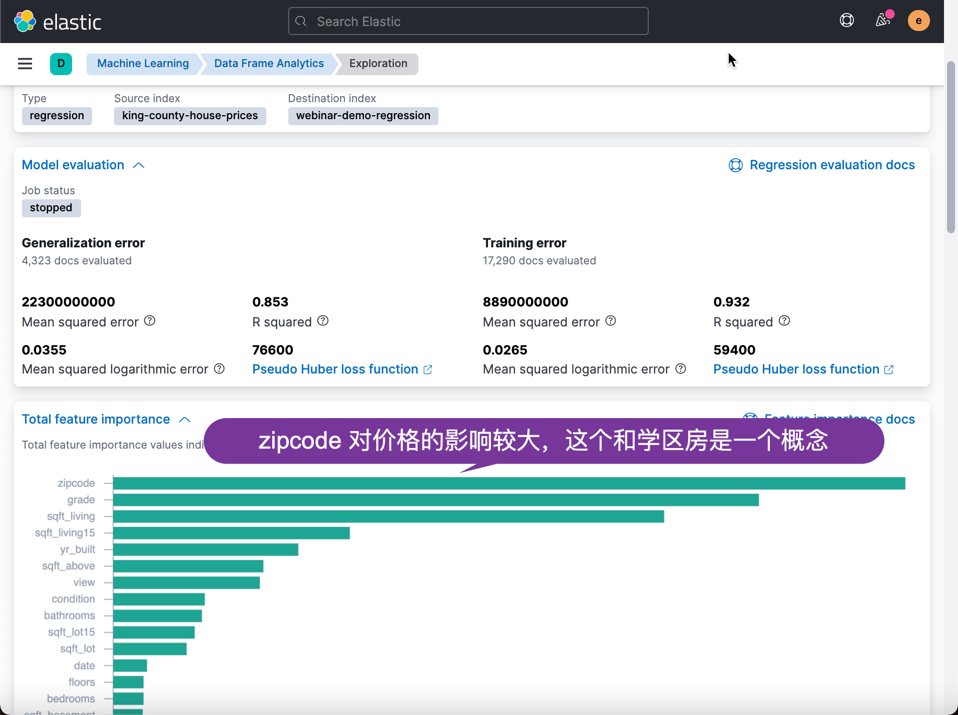
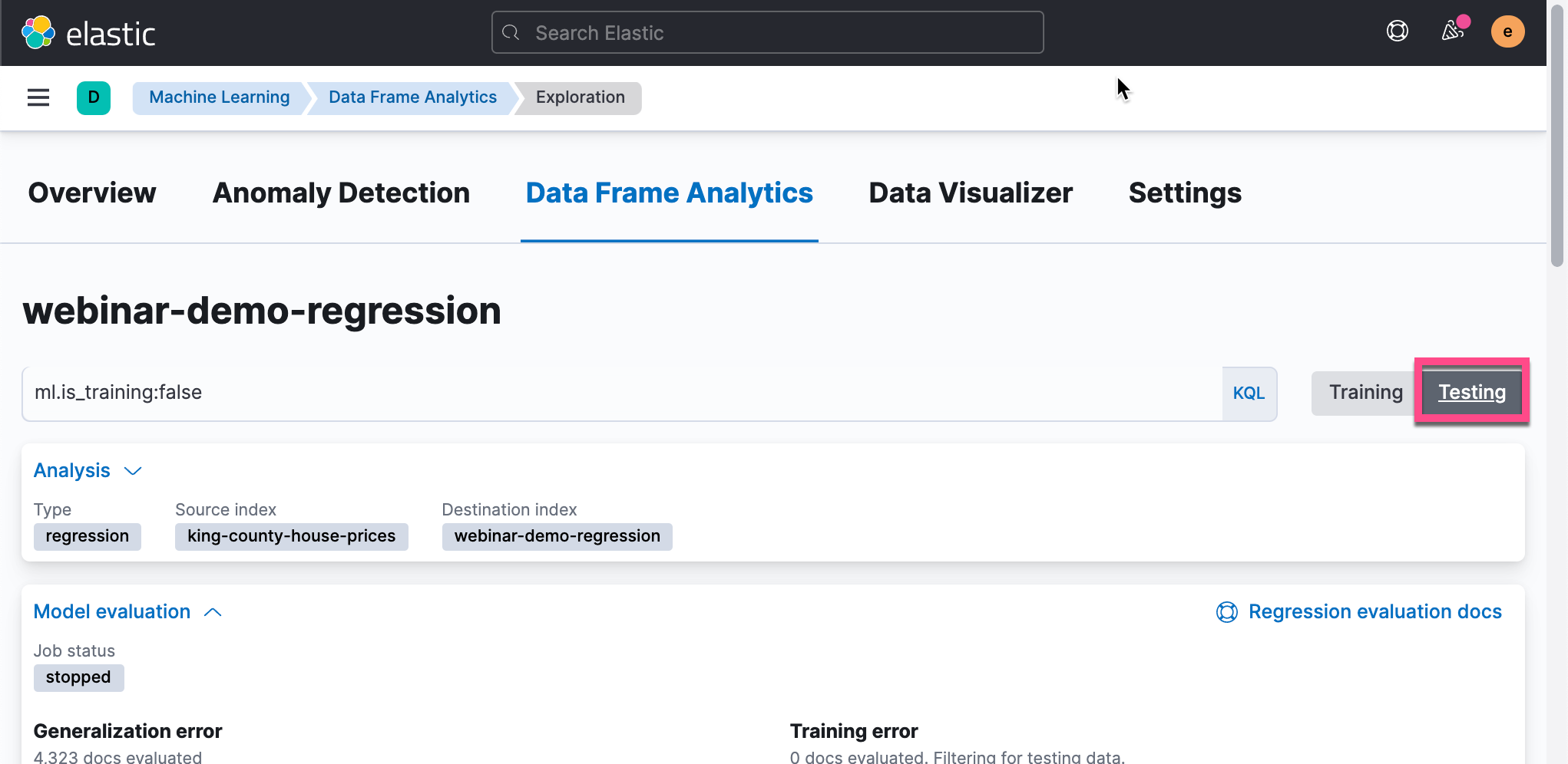
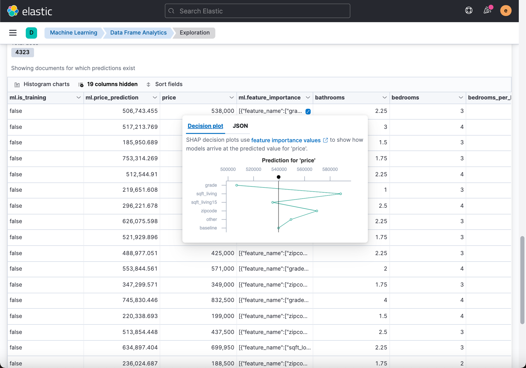
In order to verify the correctness of our model, we select the Testing dataset:
We then look at the data accuracy in the test data set:
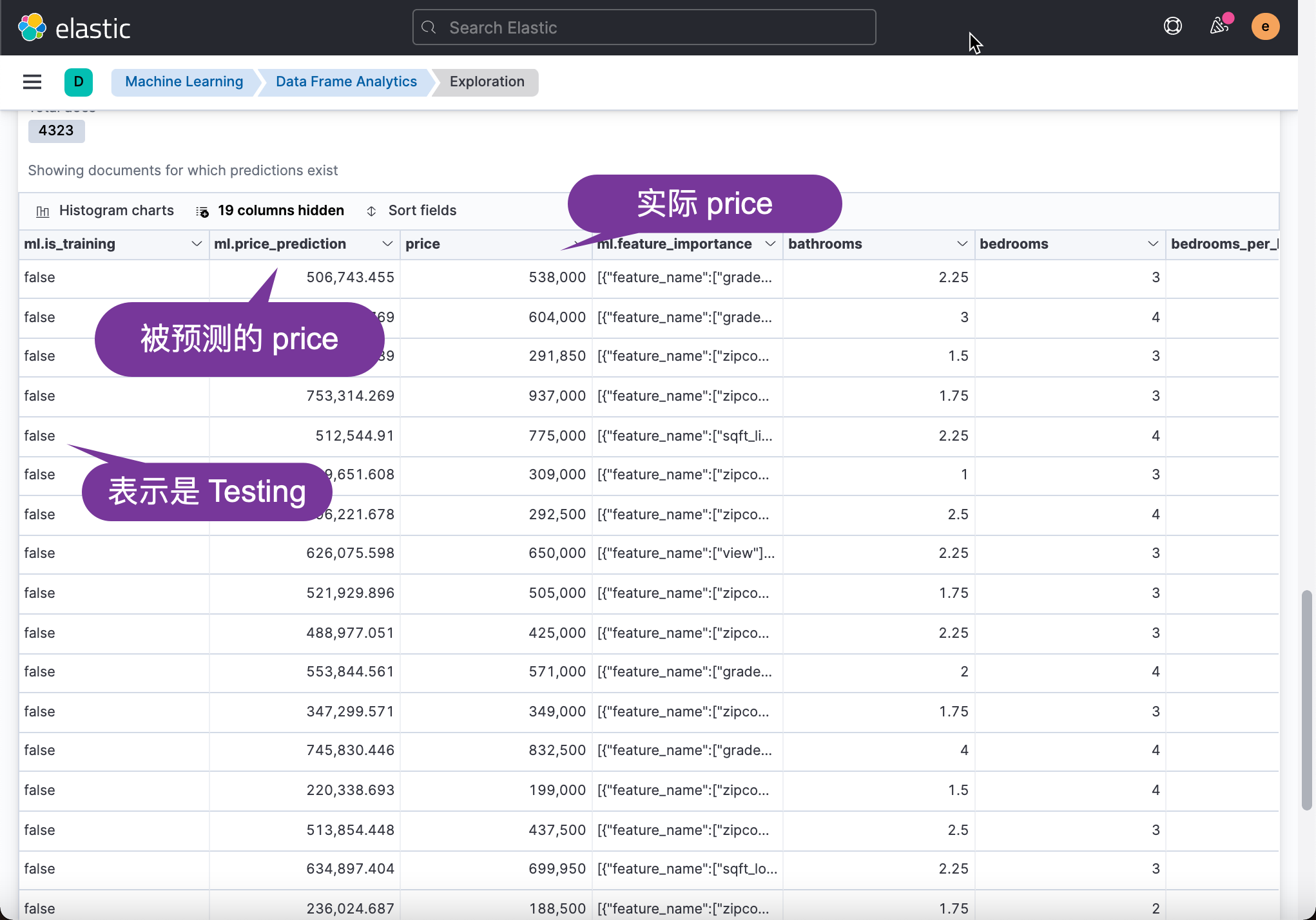
From the above table, we can see that although there are differences in some data, the vast majority of the predicted price is not very different from the actual price. We can also see the influence of some fields on price prediction from the above table:
Influence - Inference
Reasoning is a machine learning function that enables you to use supervised machine learning processes (such as expression or classification), not only as batch analysis, but also in a continuous manner. This means that reasoning can use a trained machine learning model to process the incoming data.
For example, suppose you have an online service and you want to predict whether customers may lose. You have an index containing historical data (information about customer behavior over the years in your business) and a classification model trained based on this data. The new information enters the target index of continuous transformation. Through reasoning, you can use the same input fields as the training model to perform classification analysis on new data and obtain predictions.
Let's take a closer look at the mechanism behind reasoning.
Inference processor
Influence can be used as the processor specified in the ingest pipeline. It uses a trained model to infer the data being ingested in the pipeline. The model is used for ingestion nodes. Influence preprocesses data and provides predictions by using models. After this process, the pipeline continues to execute (if there are any other processors in the pipeline) and finally indexes the new data into the target index with the result.
see inference processor And machine learning data frame analysis API document To learn more about this feature.
Inference aggregation
Influence can also be used as a pipe aggregation. You can reference the trained model in the aggregation to infer the result field of the parent bucket aggregation. Inference aggregation uses result models to provide predictions. This aggregation enables you to run region or classification analysis at search time. If you want to perform analysis on a small group of data, this aggregation allows you to generate predictions without setting up a processor in the intake pipeline.
see inference aggregation And machine learning data frame analysis API document To learn more about this feature.
View the model of machine learning
We can use the following command to view the established model:
GET _cat/ml/trained_models
The above command generates the following results:
lang_ident_model_1                    1mb 39629 2019-12-05T12:28:34.594Z 0 __none__
webinar-demo-regression-1642141570214 1mb 1456  2022-01-14T06:26:10.214Z 0 webinar-demo-regression
As shown above, we already have two models. One of them is lang_ident_mode_1 is a model contained in each Elasticsearch at present. It is used to recognize language. Interested developers can read my previous articles“ Elasticsearch: use language recognition for multilingual search in elasticsearch ”. The following webinar demo region is a model we generated above.
We can use the following command to view the contents of the above model:
GET _ml/trained_models/webinar-demo-regression*
The above command shows:
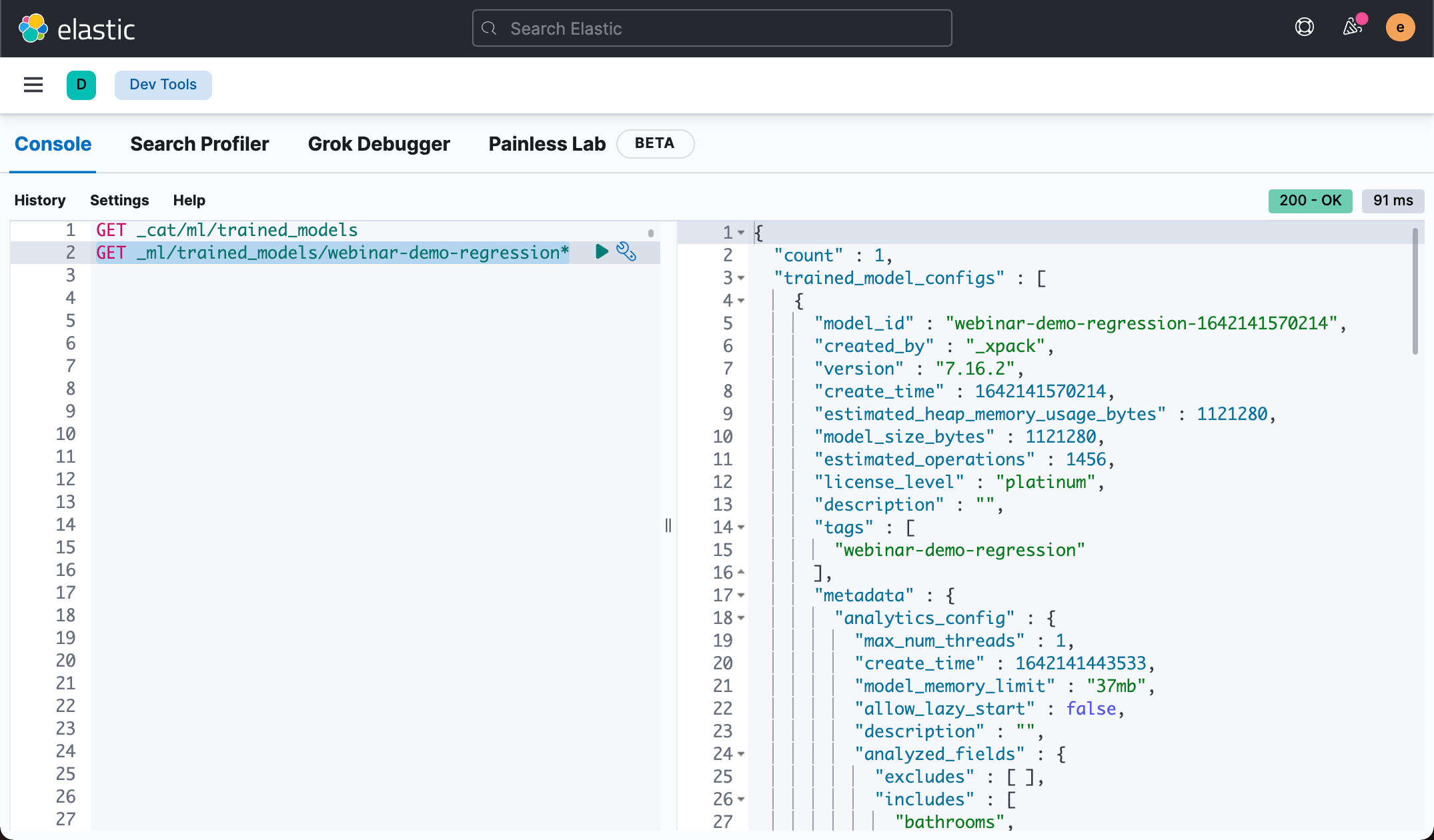
The most important information above is the model_id. This is what we need to use in the following reasoning.
Next, we use the model just created to create a pipeline based on} information processor:
# Enrichment + prediction pipeline
# NOTE: model_id will be different for your data
PUT _ingest/pipeline/house_price_predict
{
  "description": "pridicts a house price given data",
  "processors": [
    {
      "inference": {
        "model_id": "webinar-demo-regression-1642141570214",
        "inference_config": {
          "regression": {}
        },
        "field_map": {},
        "tag": "price_prediction"
      }
    }
  ]
}
Generally speaking, we can use it in the above ingest pipeline enrich pricessor To enrich our data if our data needs to be exported from the original data. In our case, we don't need it. We run the above command to produce a house_ price_ pipeline of predict.
When we ingest a data, we can use this ingest pipeline to predict our data. To test our model. We first get a document from the previous document, such as:
GET king-county-house-prices/_source/ltdgUX4BDxnvOIf6bXj3
Note that the ltdgUX4BDxnvOIf6bXj3 above is an existing document I found using Discover_ id. The document information given by the above command is:
{
  "date" : "20141013T000000",
  "yr_renovated" : 0,
  "long" : -122.257,
  "view" : 0,
  "floors" : 1.0,
  "sqft_above" : 1180,
  "sqft_living15" : 1340,
  "price" : 221900.0,
  "id" : 7129300520,
  "sqft_lot" : 5650,
  "lat" : 47.5112,
  "sqft_basement" : 0,
  "sqft_lot15" : 5650,
  "bathrooms" : 1.0,
  "bedrooms" : 3,
  "zipcode" : 98178,
  "sqft_living" : 1180,
  "condition" : 3,
  "yr_built" : 1955,
  "grade" : 7,
  "waterfront" : 0,
  "location" : "47.5112,-122.257"
}
Next, we can use the following command to test:
POST _ingest/pipeline/house_price_predict/_simulate
{
  "docs": [
    {
      "_source": {
        "date": "20141013T000000",
        "yr_renovated": 0,
        "long": -122.257,
        "view": 0,
        "floors": 1,
        "sqft_above": 1180,
        "sqft_living15": 1340,
        "price": 221900,
        "id": 7129300520,
        "sqft_lot": 5650,
        "lat": 47.5112,
        "sqft_basement": 0,
        "sqft_lot15": 5650,
        "bathrooms": 1,
        "bedrooms": 3,
        "zipcode": 98178,
        "sqft_living": 1180,
        "condition": 3,
        "yr_built": 1955,
        "grade": 7,
        "waterfront": 0,
        "location": "47.5112,-122.257"
      }
    }
  ]
}
On top_ In the source field, we directly fill in the source obtained above. By running the above command, we can get:
{
"docs" : [
{
"doc" : {
"_index" : "_index",
"_type" : "_doc",
"_id" : "_id",
"_source" : {
"date" : "20141013T000000",
"yr_renovated" : 0,
"long" : -122.257,
"view" : 0,
"floors" : 1,
"sqft_above" : 1180,
"sqft_living15" : 1340,
"price" : 221900,
"id" : 7129300520,
"sqft_lot" : 5650,
"lat" : 47.5112,
"ml" : {
"inference" : {
"price_prediction" : {
"price_prediction" : 239677.90135690733,
"feature_importance" : [
{
"feature_name" : "sqft_living",
"importance" : -86914.40339769304
},
{
"feature_name" : "grade",
"importance" : -67529.40790045598
},
{
"feature_name" : "zipcode",
"importance" : -60953.68689058545
},
{
"feature_name" : "sqft_living15",
"importance" : -27909.453510639916
}
],
"model_id" : "webinar-demo-regression-1642141570214"
}
}
},
"sqft_basement" : 0,
"sqft_lot15" : 5650,
"bathrooms" : 1,
"bedrooms" : 3,
"zipcode" : 98178,
"sqft_living" : 1180,
"condition" : 3,
"yr_built" : 1955,
"grade" : 7,
"waterfront" : 0,
"location" : "47.5112,-122.257"
},
"_ingest" : {
"timestamp" : "2022-01-17T09:11:59.48992Z"
}
}
}
]
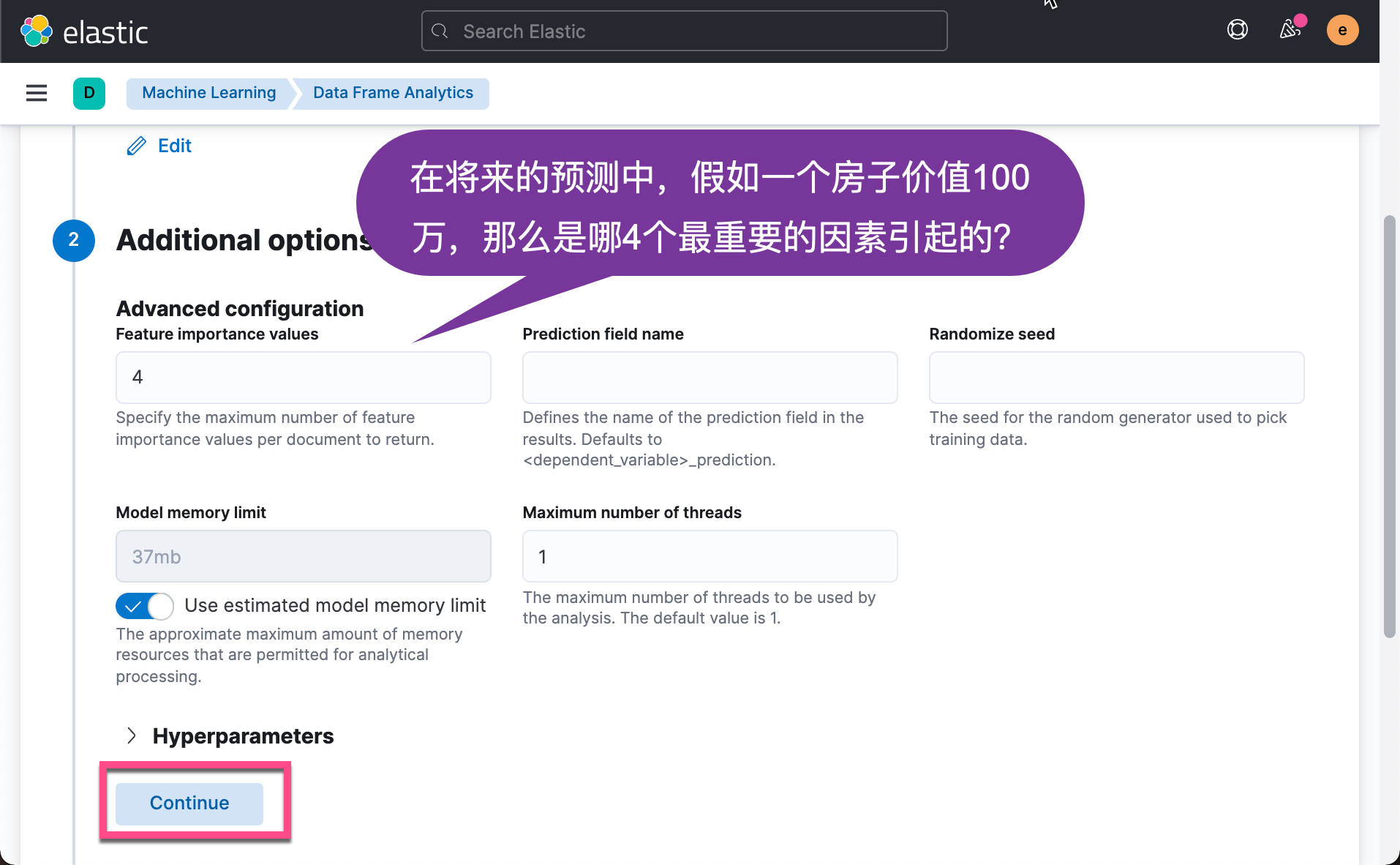
}Using the model established before, the estimated house price we obtained is "price_prediction": 239677.90135690733. It is quite close to our actual price of 221900. Feature on top_ In importance, it contains the four factors that contribute the most to the estimated price: sqft_living, grade, zipcode and sqft_living15.
Maybe you want to say that the price field is contained in the document you enter. We're down there_ Remove the price field from the source:
POST _ingest/pipeline/house_price_predict/_simulate
{
  "docs": [
    {
      "_source": {
        "date": "20141013T000000",
        "yr_renovated": 0,
        "long": -122.257,
        "view": 0,
        "floors": 1,
        "sqft_above": 1180,
        "sqft_living15": 1340,
        "id": 7129300520,
        "sqft_lot": 5650,
        "lat": 47.5112,
        "sqft_basement": 0,
        "sqft_lot15": 5650,
        "bathrooms": 1,
        "bedrooms": 3,
        "zipcode": 98178,
        "sqft_living": 1180,
        "condition": 3,
        "yr_built": 1955,
        "grade": 7,
        "waterfront": 0,
        "location": "47.5112,-122.257"
      }
    }
  ]
}
If we run the above command, we can get the same answer. In other words, we can predict the price of a house according to the model created by machine learning.
Next, let's try to fine tune some parameters, such as modifying sqft_ The value of living is 2000, so let's take a look at the final Valuation:
POST _ingest/pipeline/house_price_predict/_simulate
{
  "docs": [
    {
      "_source": {
        "date": "20141013T000000",
        "yr_renovated": 0,
        "long": -122.257,
        "view": 0,
        "floors": 1,
        "sqft_above": 1180,
        "sqft_living15": 1340,
        "id": 7129300520,
        "sqft_lot": 5650,
        "lat": 47.5112,
        "sqft_basement": 0,
        "sqft_lot15": 5650,
        "bathrooms": 1,
        "bedrooms": 3,
        "zipcode": 98178,
        "sqft_living": 2000,
        "condition": 3,
        "yr_built": 1955,
        "grade": 7,
        "waterfront": 0,
        "location": "47.5112,-122.257"
      }
    }
  ]
}
The output of the above command is:
{
  "docs" : [
    {
      "doc" : {
        "_index" : "_index",
        "_type" : "_doc",
        "_id" : "_id",
        "_source" : {
          "date" : "20141013T000000",
          "yr_renovated" : 0,
          "long" : -122.257,
          "view" : 0,
          "floors" : 1,
          "sqft_above" : 1180,
          "sqft_living15" : 1340,
          "id" : 7129300520,
          "sqft_lot" : 5650,
          "lat" : 47.5112,
          "ml" : {
            "inference" : {
              "price_prediction" : {
                "price_prediction" : 320045.53082421474,
                "feature_importance" : [
                  {
                    "feature_name" : "grade",
                    "importance" : -71221.99550030447
                  },
                  {
                    "feature_name" : "zipcode",
                    "importance" : -60646.70704720452
                  },
                  {
                    "feature_name" : "sqft_living15",
                    "importance" : -31176.143612357395
                  },
                  {
                    "feature_name" : "bathrooms",
                    "importance" : -15116.952345425949
                  }
                ],
                "model_id" : "webinar-demo-regression-1642141570214"
              }
            }
          },
          "sqft_basement" : 0,
          "sqft_lot15" : 5650,
          "bathrooms" : 1,
          "bedrooms" : 3,
          "zipcode" : 98178,
          "sqft_living" : 2000,
          "condition" : 3,
          "yr_built" : 1955,
          "grade" : 7,
          "waterfront" : 0,
          "location" : "47.5112,-122.257"
        },
        "_ingest" : {
          "timestamp" : "2022-01-17T09:20:33.93337Z"
        }
      }
    }
  ]
}
We can see that when our sqft_ When living is increased from 1180 to 2000, the valuation changes from 239677.90135690733 to 320045.53082421474. The most important factor affecting this price is grade instead of sqft_living. Maybe sqft_ When living is increased to a certain value, grade becomes more important.
summary
We used a real home sales price list in the United States. After the machine learning process of Elasticsearch, we use data frame analysis for supervised machine learning, so that we can predict the price of houses sold. In practical use, we can create real-time data processing. We can let transforms run in real time and let the data frame analysis task run continuously to update the model. For more presentations, see my other articles