Relationship Fitting (Regression)

Setting up datasets

Create some fake data to simulate the real situation. For example, a quadratic function of one variable: y = a * x^2 + b, add a little noise to the Y data to show it more realistically.

#Relationship Fitting (Regression)
import torch
from torch.autograd import Variable
import torch.nn.functional as F
import matplotlib.pyplot as plt
#fake data
x=torch.unsqueeze(torch.linspace(-1,1,100),dim=1)
#unsqueeze transforms one dimension into two dimensions
y=x.pow(2)+0.2*torch.rand(x.size())
#   Quadratic+Noise Effect

plt.scatter(x.data.numpy(),y.data.numpy())
#Scatter plot
plt.show()

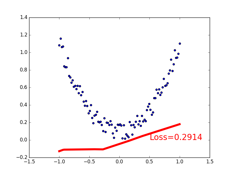
Establishing a neural network

Establishing a neural network can directly apply the torch system. First all the layer attributes (init()) are defined, then the layer-by-layer relationship links (forward(x)) are built.

#Relationship Fitting (Regression)
import torch

from torch.autograd import Variable
import torch.nn.functional as F
import matplotlib.pyplot as plt
class Net(torch.nn.Module):#Module is the main module of net
    #Two functions required to build torch
    def __init__(self,n_feature,n_hidden,n_output):#Information needed to set up the net
        super(Net,self).__init__()#Inherit net to Module module and output init function
        #Below is the layer information, which is all attributes
        self.hidden=torch.nn.Linear(n_feature,n_hidden)#How many inputs and how many outputs
        self.predict = torch.nn.Linear(n_hidden,n_output)
    def forward(self,x):#The process of forward propagation, forward propagation of input values, and neural network analysis of output values
       x=F.relu(self.hidden(x))#x outputs n_hidden through hidden, then nests with relu activation function
       x=self.predict(x)#Put the above X in predict Output Layer Output x
       #The output layer does not use the excitation function, because in most regression problems
       #In most regression problems, the predicted value is distributed from positive to negative infinity.
       #Use the excitation function to truncate the value a little, predict doesn't like the result of truncation
       return x

#Define net
#!!!!Don't hit in class
net=Net(n_feature=1,n_hidden=10,n_output=1)#x value 1, hidden layer (neuron 10), y1
print(net)


plt.ion()   #Real-time Drawing
plt.show()

#Optimize Network
optimizer=torch.optim.SGD(net.parameters(),lr=0.2)#Higher, faster
#Using optim optimizer to optimize the parameters of the neural network, the learning efficiency is 0.2
loss_func=torch.nn.MSELoss()#Mean Square Variance of MSELoss() for Optimizing Errors



#Start training
for t in  range(100):#100 steps
    prediction=net(x)#Input Information Prediction Value

    loss=loss_func(prediction,y)#Errors in prediction and y prediction

    optimizer.zero_grad()#All parameter gradients are reduced to zero
    loss.backward()#Reverse transfer to compute gradient for each neural network node
    optimizer.step()#Optimal Gradient

    if t % 5 == 0:
        # plot and show learning process
        plt.cla()
        plt.scatter(x.data.numpy(), y.data.numpy())
        plt.plot(x.data.numpy(), prediction.data.numpy(), 'r-', lw=5)
        plt.text(0.2, 0, 'Loss=%.4f' % loss.data, fontdict={'size': 20, 'color':  'red'})
        plt.pause(0.1)
plt.ioff()
plt.show()

Distinguish types (classifications)

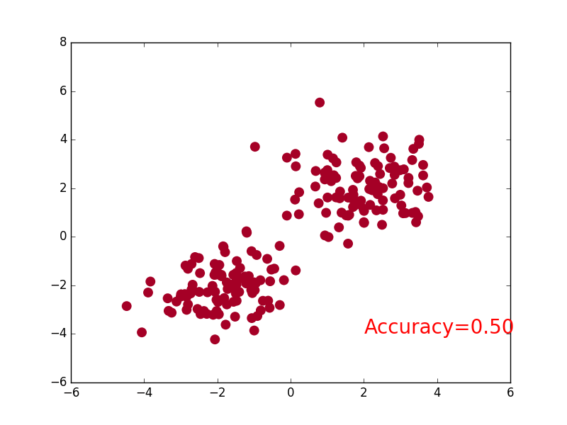
Create some fake data to simulate the real situation. For example, two quadratic distributions of data, but their mean values are different. Establish a neural network that directly uses the system in torch. Define all layer attributes (init()) first, and then build (forward(x)) layer-by-layer relationship links.
This is basically the same as the neural network used in the previous regression.

import torch
import matplotlib.pyplot as plt
import torch.nn.functional as F

# False Data
n_data = torch.ones(100, 2)         # The basic form of the data x contains a horizontal and vertical coordinate y of type
x0 = torch.normal(2*n_data, 1)      # Type 0 x data (tensor), shape=(100, 2)
y0 = torch.zeros(100)               # Label 0
x1 = torch.normal(-2*n_data, 1)     # Type 1 x data (tensor), shape=(100, 1)
y1 = torch.ones(100)                # Label 1

# Note that x, y data must be in the form of the following (torch.cat is merging data)
x = torch.cat((x0, x1), 0).type(torch.FloatTensor)  #The data must be FloatTensor = 32-bit floating
            #x Merge together to make data

y = torch.cat((y0, y1), ).type(torch.LongTensor)    # Label must be LongTensor = 64-bit integer
            # y merge together to label 0.
# plt.scatter(x.data.numpy()[:, 0], x.data.numpy()[:, 1], c=y.data.numpy(), s=100, lw=0, cmap='RdYlGn')
# plt.show()



class Net(torch.nn.Module):     # Module inheriting torch
    def __init__(self, n_feature, n_hidden, n_output):
        super(Net, self).__init__()     # Inherit u init_u Function
        self.hidden = torch.nn.Linear(n_feature, n_hidden)   # Hidden Layer Linear Output
        self.out = torch.nn.Linear(n_hidden, n_output)       # Output Layer Linear Output

    def forward(self, x):
        # Forward propagation of input values and output values from neural network analysis
        x = F.relu(self.hidden(x))      # Excitation Function (Linear Value of Hidden Layer)
        x = self.out(x)                 # Output value, but this is not a predicted value and the predicted value needs to be calculated
        return x

net = Net(n_feature=2, n_hidden=10, n_output=2) # Several categories are just a few output s
        #The x input is 2 features (x, y coordinates) and the output is 2 features (0 and you)

print(net)  # The structure of net

# optimizer is a training tool
optimizer = torch.optim.SGD(net.parameters(), lr=0.02)  # All parameters passed into net, learning rate
loss_func = torch.nn.CrossEntropyLoss()
#CrossEntropyLoss() Action Label Value: [0,0,1] Predictive Value: [0.1,0.3,0.6] Error between the two

plt.ion()   # Drawing
plt.show()

for t in range(100):
    out = net(x)     # Feed net training data x, output analysis value

    loss = loss_func(out, y)     # Calculating the Error of Both

    optimizer.zero_grad()   # Empty the remaining update parameter values from the previous step
    loss.backward()         # Error back-propagation, calculating parameter update values
    optimizer.step()        # Applying parameter update values to net's parameters


    if t % 2 == 0:
        plt.cla()
        prediction = torch.max(out, 1)[1]
        #The location of the maximum value is where the index is 1
        pred_y = prediction.data.numpy().squeeze()
        target_y = y.data.numpy()
        plt.scatter(x.data.numpy()[:, 0], x.data.numpy()[:, 1], c=pred_y, s=100, lw=0, cmap='RdYlGn')
        accuracy = float((pred_y == target_y).astype(int).sum()) / float(target_y.size)
        plt.text(1.5, -4, 'Accuracy=%.2f' % accuracy, fontdict={'size': 20, 'color': 'red'})

        plt.pause(0.1)

plt.ioff()  # Stop drawing
plt.show()

Quick build

The method used in regression inherits a torch's neural network structure with class, then modifies it to quickly build and summarize all of the above in one sentence!

class Net(torch.nn.Module):
    def __init__(self, n_feature, n_hidden, n_output):
        super(Net, self).__init__()
        self.hidden = torch.nn.Linear(n_feature, n_hidden)
        self.predict = torch.nn.Linear(n_hidden, n_output)

    def forward(self, x):
        x = F.relu(self.hidden(x))
        x = self.predict(x)
        return x

net1 = Net(1, 10, 1)   # This is how we built net1

Quick build

net2 = torch.nn.Sequential(
    torch.nn.Linear(1, 10),
    torch.nn.ReLU(),
    torch.nn.Linear(10, 1)
)


print(net1)
"""
Net (
  (hidden): Linear (1 -> 10)
  (predict): Linear (10 -> 1)
)
"""
print(net2)
"""
Sequential (
  (0): Linear (1 -> 10)
  (1): ReLU ()
  (2): Linear (10 -> 1)
)
"""

net2 also includes the excitation function, but in net1, the excitation function is actually called in the forward() function.
This also shows that the advantage of Net1 over net2 is that you can personalize your own forward communication process, such as (RNN), to suit your personal needs.
However, net2 is more appropriate if you don't need a seven-eighty-eight process.

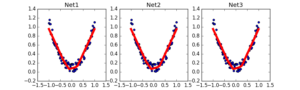
Save Extraction

A model has been trained and we want to save it so that we can use it directly the next time we want to use it. Here we use a regressed neural network as an example to save and extract.
A torch.save(net1,'net.pkl') that holds the entire neural network
A parameter torch.save(net1.state_dict(),'net_params.pkl') that stores neural networks

import torch

import matplotlib.pyplot as plt

#fake data
x = torch.unsqueeze(torch.linspace(-1, 1, 100), dim=1)
#unsqueeze transforms one dimension into two dimensions
y = x.pow(2) + 0.2*torch.rand(x.size())
#   Quadratic+Noise Effect


#Save data
def save():
    #Build a network
    net1=torch.nn.Sequential(
        torch.nn.Linear(1,10),
        torch.nn.ReLU(),
        torch.nn.Linear(10,1)
    )
    #Optimize Network
    optimizer=torch.optim.SGD(net1.parameters(),lr=0.2)
    loss_func=torch.nn.MSELoss()

    # Start training
    for t in range(100):  # 100 steps
        prediction =net1(x)  # Input Information Prediction Value
        loss = loss_func(prediction, y)  # Errors in prediction and y prediction
        optimizer.zero_grad()  # All parameter ladder loss = loss_func(prediction, y) degree reduced to 0
        loss.backward()  # Reverse transfer to compute gradient for each neural network node
        optimizer.step()  # Optimal Gradient

     # Mapping
    plt.figure(1, figsize=(10, 3))
    plt.subplot(131)
    plt.title('Net1')
    plt.scatter(x.data.numpy(), y.data.numpy())
    plt.plot(x.data.numpy(), prediction.data.numpy(), 'r-', lw=5)

    torch.save(net1,'net.pkl')#Save the entire neural network
                    #Saved Name
    torch.save(net1.state_dict(),'net_params.pkl')#Save parameters of the entire neural network

def restore_net():
    net2=torch.load('net.pkl')
    prediction=net2(x)
    # Mapping

    plt.subplot(132)
    plt.title('Net2')
    plt.scatter(x.data.numpy(), y.data.numpy())
    plt.plot(x.data.numpy(), prediction.data.numpy(), 'r-', lw=5)

def restore_parames():
    #To extract parameters from net3, a network like net1 must be built first
    #Then copy the parameters of net1 to net3
    net3 = torch.nn.Sequential(
        torch.nn.Linear(1, 10),
        torch.nn.ReLU(),
        torch.nn.Linear(10, 1)
    )#But the parameters inside are definitely different
    net3.load_state_dict(torch.load('net_params.pkl'))
    prediction=net3(x)
    # Mapping

    plt.subplot(133)
    plt.title('Net3')
    plt.scatter(x.data.numpy(), y.data.numpy())
    plt.plot(x.data.numpy(), prediction.data.numpy(), 'r-', lw=5)
    plt.show()


save()

restore_net()

restore_parames()

Batch Training

DataLoader

DataLoader is the tool torch gives you to wrap your data. So swap your own (numpy array or other) data format into Tensor and put it in this wrapper. DataLoader helps you iterate through your data effectively.

#Batch Processing
import torch
import torch.utils.data as Data

BATCH_SIZE=5#A stack of data is divided into five groups and five groups

x=torch.linspace(1,10,10)#Divide from 1 to 10 into 10 points
y=torch.linspace(10,1,10)#From 10 to 1.

#Define a database
torch_dataset=Data.TensorDataset(x,y)#x training data y target data
#Use loader to turn training into a small batch
loader=Data.DataLoader(
    dataset=torch_dataset,
    batch_size=BATCH_SIZE,
    shuffle=True,#Do not randomly shuffle data during training and start sampling false again as no shuffling

)

for epoch in range(3):#Training these 10 data three times as a whole
    for step,(batch_x,batch_y) in enumerate(loader):#Total training 3 times Each training is divided into 2 parts
        #The loader defines whether to shuffle the data without shuffling the data. The form of each training is the same: training data point 1 before training data point 2.
        #enumerate gives him an index each time it extracts. The first step is
        #training
        print('Epoch: ', epoch, '| Step: ', step, '| batch x: ',
              batch_x.numpy(), '| batch y: ', batch_y.numpy())
. . . 
Epoch:  0 | Step:  0 | batch x:  [3. 5. 1. 4. 8.] | batch y:  [ 8.  6. 10.  7.  3.]
Epoch:  0 | Step:  1 | batch x:  [ 2.  6. 10.  9.  7.] | batch y:  [9. 5. 1. 2. 4.]
Epoch:  1 | Step:  0 | batch x:  [ 4.  2.  6.  7. 10.] | batch y:  [7. 9. 5. 4. 1.]
Epoch:  1 | Step:  1 | batch x:  [9. 5. 8. 1. 3.] | batch y:  [ 2.  6.  3. 10.  8.]
Epoch:  2 | Step:  0 | batch x:  [4. 7. 6. 2. 8.] | batch y:  [7. 4. 5. 9. 3.]
Epoch:  2 | Step:  1 | batch x:  [10.  9.  1.  3.  5.] | batch y:  [ 1.  2. 10.  8.  6.]

If BATCH_SIZE=5 is changed to 8 output

Epoch:  0 | Step:  0 | batch x:  [2. 1. 5. 9. 7. 8. 4. 6.] | batch y:  [ 9. 10.  6.  2.  4.  3.  7.  5.]
Epoch:  0 | Step:  1 | batch x:  [10.  3.] | batch y:  [1. 8.]
Epoch:  1 | Step:  0 | batch x:  [4. 8. 6. 7. 1. 3. 2. 9.] | batch y:  [ 7.  3.  5.  4. 10.  8.  9.  2.]
Epoch:  1 | Step:  1 | batch x:  [ 5. 10.] | batch y:  [6. 1.]
Epoch:  2 | Step:  0 | batch x:  [ 3.  5.  9.  7. 10.  4.  6.  1.] | batch y:  [ 8.  6.  2.  4.  1.  7.  5. 10.]
Epoch:  2 | Step:  1 | batch x:  [2. 8.] | batch y:  [9. 3.]

Only the data left in this epoch will be returned to you at step=1

Optimizer

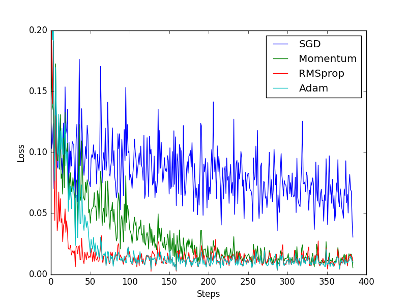
SGD is the most common optimizer, or has no acceleration effect, while Momentum is an improved version of SGD that incorporates a momentum principle.
The following RMprop is an upgrade of Momentum, while Adam is an upgrade of RMSprop.
However, from this result we can see that Adam seems to be less effective than RMSprop. So the more advanced the optimizer, the better the result.
We can try different optimizers in our own experiment to find the one that best suits your data/network.

import torch
import torch.utils.data as Data
import torch.nn.functional as F
from torch.autograd import Variable
import matplotlib.pyplot as plt

#Hyperparameter
LR=0.01
BATCH_SIZE=32
EPOCH=12

#Regressed data
x = torch.unsqueeze(torch.linspace(-1, 1, 1000), dim=1)
y = x.pow(2) + 0.1*torch.normal(torch.zeros(*x.size()))

# plt.scatter(x.numpy(),y.numpy())
# plt.show()

#Define a database
torch_dataset=Data.TensorDataset(x,y)
loader=Data.DataLoader(
    dataset=torch_dataset,
    batch_size=BATCH_SIZE,
    shuffle=True,
    num_workers=2,#Work Process
)

#Establishing a neural network
class Net(torch.nn.Module):
    def __init__(self):
        super(Net,self).__init__()
        self.hidden=torch.nn.Linear(1,20)#Hidden Layer
        self.predict=torch.nn.Linear(20,1)#output layer
    def forward(self,x):
        x=F.relu(self.hidden(x))
        x=self.predict(x)
        return x
#Four different neural networks
if __name__ == '__main__':
    net_SGD = Net()
    net_Momentum= Net()
    net_RMSprop= Net()
    net_Adam= Net()
    nets = [net_SGD, net_Momentum, net_RMSprop, net_Adam]

    opt_SGD= torch.optim.SGD(net_SGD.parameters(), lr=LR)
    opt_Momentum= torch.optim.SGD(net_Momentum.parameters(), lr=LR, momentum=0.8)
    opt_RMSprop= torch.optim.RMSprop(net_RMSprop.parameters(), lr=LR, alpha=0.9)
    opt_Adam= torch.optim.Adam(net_Adam.parameters(), lr=LR, betas=(0.9, 0.99))
    optimizers=[opt_SGD, opt_Momentum, opt_RMSprop, opt_Adam]

    #Start training
    loss_func = torch.nn.MSELoss()#Error calculation formula for regression
    losses_his = [[], [], [], []]   # loss of different neural networks when recording training s

    for epoch in range(EPOCH):
        print('Epoch: ', epoch)
        for step, (b_x, b_y) in enumerate(loader):
        #Take out the different neural networks one by one
          for net, opt, l_his in zip(nets, optimizers, losses_his):
              output = net(b_x)  # Input Information Prediction Value
              loss = loss_func(output, b_y)  # Errors in prediction and y prediction

              opt.zero_grad()   # All parameter gradients are reduced to zero
              loss.backward()  # Reverse transfer to compute gradient for each neural network node
              opt.step()  # Optimal Gradient
              l_his.append(loss.data.numpy())#Put errors in the record
    #Print
    labels = ['SGD', 'Momentum', 'RMSprop', 'Adam']
    for i, l_his in enumerate(losses_his):
        plt.plot(l_his, label=labels[i])
    plt.legend(loc='best')
    plt.xlabel('Steps')
    plt.ylabel('Loss')
    plt.ylim((0, 0.2))
    plt.show()