Experimental trimer analysis
1, Experimental purpose
This experimental course is a professional course for students majoring in computer, artificial intelligence and software engineering. Through experiments, it helps students better master the concepts, technologies, principles and applications related to data mining and machine learning; Improve students' ability to write experimental reports and summarize experimental results through experiments; Enable students to have a more in-depth understanding of machine learning models and algorithms. The knowledge points to be mastered are as follows:
- Master relevant concepts, models and algorithms involved in machine learning;
- Familiar with the process of machine learning model training, verification and testing;
- Familiar with common data preprocessing methods;
- Master the representation, solution and programming of cluster analysis problems.
2, Basic requirements
- Before the experiment, review the relevant contents in the course of data mining and machine learning.
- Prepare the experimental data, complete the experimental content by programming, and collect the experimental results.
- Complete the experiment report independently.
3, Experimental software
It is recommended to use Python programming language (numpy library is allowed, detailed experimental steps need to be implemented, and it is not allowed to directly call high-level API s such as regression, classification and clustering in scikit learn).
4, Experiment content:
Based on IRIS iris IRIS data set, complete the cluster analysis of IRIS iris.
1 prepare data sets and recognize data
Download IRIS dataset
https://archive.ics.uci.edu/ml/datasets/iris
Understand the meaning of each dimension feature of the dataset
2 explore data and preprocess data
Observe the numerical type and distribution of each dimension feature of the dataset
The two-dimensional features of sepal length and petal length are selected as the clustering basis
3 solve the cluster center
Programming k-means clustering and Gaussian mixture clustering
4 test and evaluation model
Calculate the performance index of clustering on the data set
5, Student experiment report
(1) This paper briefly introduces the principle of k-means and Gaussian mixture clustering
k-means principle:
k-means algorithm is a commonly used clustering algorithm. The input of the algorithm is a sample set (point set). Through this algorithm, the samples can be clustered and the samples with similar characteristics can be clustered into one class.
Algorithm idea:
Suppose we want to divide the data into K classes, it can be divided into the following steps:
1. k points are randomly selected as clustering centers
2 calculate the distance from each point to k cluster centers, and then assign the point to the nearest center, so as to form k clusters
3. Then recalculate the centroid (mean) of each cluster
4. Repeat steps 2-3 until the position of the centroid does not change or reaches the set number of iterations
Gaussian mixture clustering principle:
① Suppose that the observation data y1,y2,..., yN are generated by Gaussian mixture model, i.e
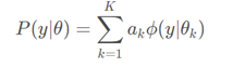
among

We use EM algorithm to estimate the parameters of Gaussian mixture model θ
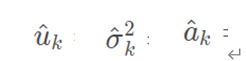
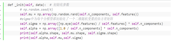
② Initialize model parameters:
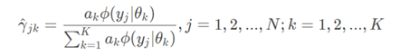
③ Step E of EM algorithm:
calculation
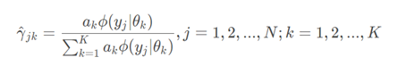
(somewhat equivalent to calculating a posteriori probability in naive Bayes, multiplying a priori probability by conditional probability)
This is the probability that the j-th observation data under the current model parameters comes from the k-th sub model, which is called the influence degree of sub model K on the observation data yj
④ Step M of EM algorithm: update model parameters
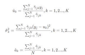
Repeat steps E and M until the model converges
(2) Program list (including detailed solution steps)
k-means clustering algorithm:
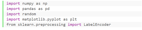
① Library to be imported
② Import the dataset and observe the data characteristics

③ Select the two-dimensional features of sepal length and petal length as the clustering basis, assign the value of category 'class' column to labels, and encode the label

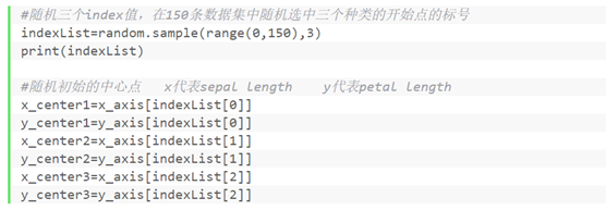
④ Initialize cluster center
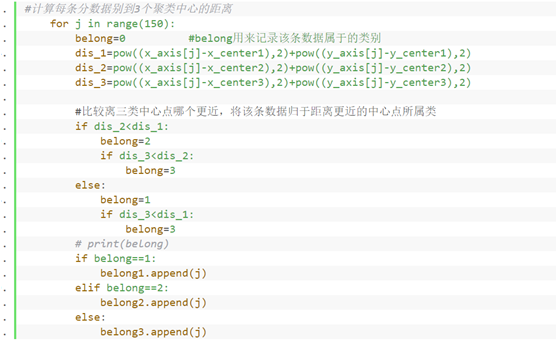
⑤ Start training: calculate the distance from each point to k cluster centers, and then assign the point to the nearest center
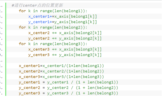
⑥ Recalculate the centroid (mean) of each cluster
⑦ Iteration steps ⑤ and ⑥ max_iter=1000 times
⑧ It shows the clustering of k-means algorithm and the classification of actual data
⑨ Calculation accuracy (because the clustering algorithm only divides the original data samples into K clusters, but does not tell us which category each cluster corresponds to, we use the arrangement and combination method to calculate the accuracy of each case, and select the highest as the final accuracy value)


Gaussian mixture algorithm:
① Library to import
② Import the dataset and observe the data characteristics

③ The two-dimensional features of sepal length and petal length are selected as the clustering basis, and the two columns of data are stored with data. labels stores the value of the 'class' column of the category and encodes the label
④ Instantiation class GMM_EM object gmm
Execution class__ init__ Function to determine that the number of clusters is 3, that is, n_components=3

⑤ Call fit in object gmm_ Predict function to get the clustering results using Gaussian mixture model

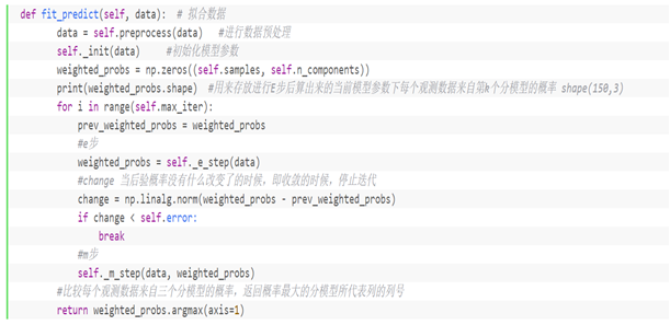
Analysis fit_ Steps in the predict (data) function:
1 'perform data preprocessing and call the in class function preprocess()
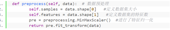
The size of the data dataset is 150 and the number of features is 2
2 'call function in class_ init() initializes the parameters of the Gaussian model
3 'at max_ When the ITER iteration times are 1000, execute steps E and M in the EM algorithm. When the change of the probability of the last two iterations is less than 1e-6, you can jump out of the iteration
Function matching algorithm of step E
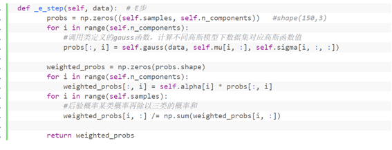
_ e_ The guass() function called in step() function is defined as follows:

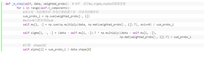
Function corresponding algorithm of Step M:

⑥ Solving the clustering center of Gaussian mixture model

⑦ The graph shows the clustering and center point of k-means algorithm, as well as the classification of actual data
⑧ The calculation accuracy is the same as that in K-means
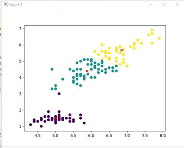
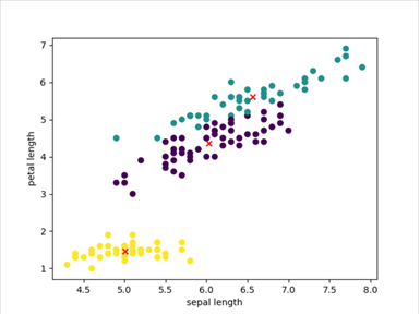
(3) Display the experimental results and visualize the clustering results
k-means algorithm:
Clustering of k-means algorithm:
Actual classification of data:
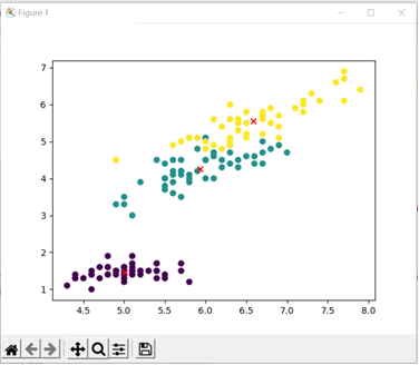
The accuracy of the clustering algorithm is:

Gaussian mixture algorithm: (EM algorithm is sensitive to the initial value. If you modify the initial value, you will find that the performance of the model changes greatly)
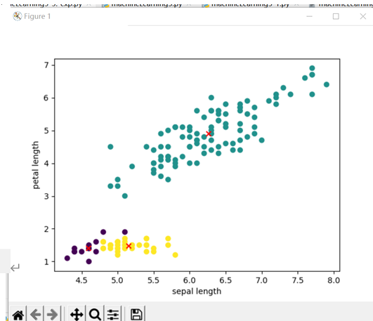

Fix a random case with good classification:

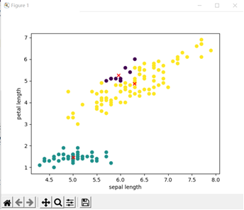
At this time, the clustering of Gaussian mixture algorithm:
Actual classification of data:

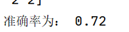
At this time, the accuracy of the clustering algorithm is:

(4) The experimental results are discussed, and the relationship between the number of k-means clusters and clustering indexes is analyzed
When coding according to the iris data set, I first default the number of clusters to 3, and many operations in the code are fixed. For the number of clusters of 3, the code is very inflexible, so the relationship analysis in this section can not be made.
I searched the relationship between the number of k-means clusters and clustering indicators on the Internet, but the information found can not be understood and analyzed. For the determination of the number of k-means clusters, the relevant information is that the k value of the number of k-means clusters is difficult to estimate, and it is uncertain how many classes are the most appropriate.
(5) Source code
k-means
import numpy as np
import pandas as pd
import random
import matplotlib.pyplot as plt
from sklearn.preprocessing import LabelEncoder
iris_data=pd.read_csv("Iris/iris.data",header=None,names=['sepal length','sepal width','petal length',
'petal width','class'])
print(iris_data.info())
#Three types of iris setosa, iris versicolor and iris Virginia were found
print(iris_data['class'].value_counts())
#Encode labels
labels=iris_data['class'].values
label_encoder=LabelEncoder()
labels=label_encoder.fit_transform(labels)
# print(labels)
#The two-dimensional features of sepal length and petal length are selected as the clustering basis
x_axis=iris_data['sepal length'] #series(150,)
y_axis=iris_data['petal length']
print(x_axis.shape)
print(y_axis.shape)
#Randomly select three index values, and randomly select the labels of the starting points of three categories in the 150 data sets
indexList=random.sample(range(0,150),3)
print(indexList)
#Random initial center point
x_center1=x_axis[indexList[0]]
y_center1=y_axis[indexList[0]]
x_center2=x_axis[indexList[1]]
y_center2=y_axis[indexList[1]]
x_center3=x_axis[indexList[2]]
y_center3=y_axis[indexList[2]]
print(x_center1)
print(x_axis[0])
#---------------------Start training 100 times-------------------------
for i in range(100):
# The index value used to hold data belonging to three categories
belong1 = []
belong2 = []
belong3 = []
#Calculate the distance from each sub data to three cluster centers
for j in range(150):
belong=0 #Bel ong is used to record the category to which this piece of data belong s
dis_1=pow((x_axis[j]-x_center1),2)+pow((y_axis[j]-y_center1),2)
dis_2=pow((x_axis[j]-x_center2),2)+pow((y_axis[j]-y_center2),2)
dis_3=pow((x_axis[j]-x_center3),2)+pow((y_axis[j]-y_center3),2)
#Compare which is closer to the center point of the three categories, and classify the data into the category of the center point closer
if dis_2<dis_1:
belong=2
if dis_3<dis_2:
belong=3
else:
belong=1
if dis_3<dis_1:
belong=3
# print(belong)
if belong==1:
belong1.append(j)
elif belong==2:
belong2.append(j)
else:
belong3.append(j)
#Update the location of center points
for k in range(len(belong1)):
x_center1+=x_axis[belong1[k]]
y_center1+=y_axis[belong1[k]]
for k in range(len(belong2)):
x_center2 += x_axis[belong2[k]]
y_center2 += y_axis[belong2[k]]
for k in range(len(belong3)):
x_center3 += x_axis[belong3[k]]
y_center3 += y_axis[belong3[k]]
x_center1=x_center1/(1+len(belong1))
x_center2=x_center2/(1+len(belong2))
x_center3=x_center3/(1+len(belong3))
y_center1 = y_center1 / (1 + len(belong1))
y_center2 = y_center2 / (1 + len(belong2))
y_center3 = y_center3 / (1 + len(belong3))
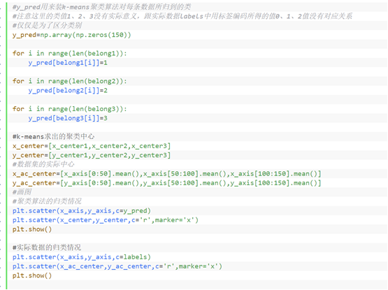
#y_pred is used to install the class to which each data belongs by k-means clustering algorithm
#Note that the class values 1, 2 and 3 here have no practical significance and have no corresponding relationship with the values 0, 1 and 2 encoded by tags in the actual data labels
#Just to distinguish categories
y_pred=np.array(np.zeros(150))
for i in range(len(belong1)):
y_pred[belong1[i]]=1
for i in range(len(belong2)):
y_pred[belong2[i]]=2
for i in range(len(belong3)):
y_pred[belong3[i]]=3
#Clustering center calculated by k-means
x_center=[x_center1,x_center2,x_center3]
y_center=[y_center1,y_center2,y_center3]
#Actual center of dataset
x_ac_center=[x_axis[0:50].mean(),x_axis[50:100].mean(),x_axis[100:150].mean()]
y_ac_center=[y_axis[0:50].mean(),y_axis[50:100].mean(),y_axis[100:150].mean()]
#Drawing
#Classification of clustering algorithm
plt.scatter(x_axis,y_axis,c=y_pred)
plt.scatter(x_center,y_center,c='r',marker='x')
plt.show()
#Classification of actual data
plt.scatter(x_axis,y_axis,c=labels)
plt.scatter(x_ac_center,y_ac_center,c='r',marker='x')
plt.show()
#Calculation accuracy
#Calculate the three category combinations 0 1 2 1 0 2 0 2 1 1 2 0 2 1 0 2 0 2 0 2 0 1
y_pred_1=np.array(np.zeros(150))
y_pred_2=np.array(np.zeros(150))
y_pred_3=np.array(np.zeros(150))
y_pred_4=np.array(np.zeros(150))
y_pred_5=np.array(np.zeros(150))
y_pred_6=np.array(np.zeros(150))
for i in range(150):
if y_pred[i]==1:
y_pred_1[i]=0
y_pred_2[i] = 1
y_pred_3[i] = 0
y_pred_4[i] = 1
y_pred_5[i] = 2
y_pred_6[i] = 2
if y_pred[i]==2:
y_pred_1[i] = 1
y_pred_2[i] = 0
y_pred_3[i] = 2
y_pred_4[i] = 2
y_pred_5[i] = 1
y_pred_6[i] = 0
if y_pred[i]==3:
y_pred_1[i] = 2
y_pred_2[i] = 2
y_pred_3[i] = 1
y_pred_4[i] = 0
y_pred_5[i] = 0
y_pred_6[i] = 1
def correct_rate(lei_list):
correct_num = 0
for i in range(150):
if (lei_list[i] == labels[i]):
correct_num += 1
rate = correct_num / 150
return rate
rate1=correct_rate(y_pred_1)
rate2=correct_rate(y_pred_2)
rate3=correct_rate(y_pred_3)
rate4=correct_rate(y_pred_4)
rate5=correct_rate(y_pred_5)
rate6=correct_rate(y_pred_6)
#compare
rate=[rate1,rate2,rate3,rate4,rate5,rate6]
max_rate=0
for i in range(6):
if rate[i]>max_rate:
max_rate=rate[i]
print('The accuracy is:',max_rate)
Gaussian mixture clustering:
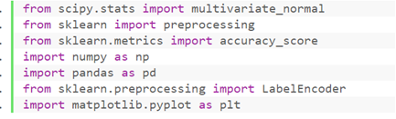
from scipy.stats import multivariate_normal
from sklearn import preprocessing
from sklearn.metrics import accuracy_score
import numpy as np
import pandas as pd
from sklearn.preprocessing import LabelEncoder
import matplotlib.pyplot as plt
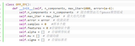
class GMM_EM():
def __init__(self, n_components, max_iter=1000, error=1e-6):
self.n_components = n_components # The hybrid model consists of several gauss models
self.max_iter = max_iter # Maximum number of iterations
self.error = error # Convergence error
self.samples = 0 #Number of samples
self.features = 0 #Number of stored features
self.alpha = [] # Storage model weights
self.mu = [] # Storage mean
self.sigma = [] # Storage standard deviation
def _init(self, data): # Initialization parameters
np.random.seed(4)
self.mu = np.array(np.random.rand(self.n_components, self.features))
#sigma initializes a covariance matrix of two-dimensional random variables for each sub model
self.sigma = np.array([np.eye(self.features) / self.features] * self.n_components)
self.alpha = np.array([1.0 / self.n_components] * self.n_components)
print(self.alpha.shape, self.mu.shape, self.sigma.shape)
print(self.alpha,self.mu,self.sigma)
def gauss(self, Y, mu, sigma): # Directly call the probability density function of multivariate normal distribution to calculate the value of Gaussian function
return multivariate_normal.pdf(Y,mean=mu, cov=sigma )
def preprocess(self, data): # Data preprocessing
self.samples = data.shape[0] #Define dataset size
self.features = data.shape[1] #Defines the number of features of the dataset
pre = preprocessing.MinMaxScaler() #Feature normalization is carried out
return pre.fit_transform(data)
def fit_predict(self, data): # Fitting data
data = self.preprocess(data) #Data preprocessing
self._init(data) #Initialize model parameters
weighted_probs = np.zeros((self.samples, self.n_components))
print(weighted_probs.shape) #It is used to store the probability shape(150,3) of each observation data from the k th sub model under the current model parameters calculated after step E
for i in range(self.max_iter):
prev_weighted_probs = weighted_probs
#Step e
weighted_probs = self._e_step(data)
#When there is no change in the a posteriori probability, that is, when it converges, stop the iteration
change = np.linalg.norm(weighted_probs - prev_weighted_probs)
if change < self.error:
break
#Step m
self._m_step(data, weighted_probs)
#Compare the probabilities of each observation data from three sub models, and return the column number of the column represented by the sub model with the highest probability
return weighted_probs.argmax(axis=1)
def _e_step(self, data): # Step E
probs = np.zeros((self.samples, self.n_components)) #shape(150,3)
for i in range(self.n_components):
#Call the gauss function defined by the class to calculate the corresponding Gaussian function value of the data set under different Gaussian models
probs[:, i] = self.gauss(data, self.mu[i, :], self.sigma[i, :, :])
weighted_probs = np.zeros(probs.shape)
for i in range(self.n_components):
weighted_probs[:, i] = self.alpha[i] * probs[:, i]
for i in range(self.samples):
#A posteriori probability the probability of a class divided by the sum of the probabilities of three classes
weighted_probs[i, :] /= np.sum(weighted_probs[i, :])
return weighted_probs
def _m_step(self, data, weighted_probs): # In step M, update the values of mu, sigma and alpha
for i in range(self.n_components):
#Calculate the probability sum of each column, that is, the probability sum of each row of data belonging to a specific class
sum_probs_i = np.sum(weighted_probs[:, i])
#axis=0 calculates sum for each column
self.mu[i, :] = np.sum(np.multiply(data, np.mat(weighted_probs[:, i]).T), axis=0) / sum_probs_i
self.sigma[i, :, :] = (data - self.mu[i, :]).T * np.multiply((data - self.mu[i, :]),
np.mat(weighted_probs[:, i]).T) / sum_probs_i
#Number of rows shape[0]
self.alpha[i] = sum_probs_i / data.shape[0]
iris_data=pd.read_csv("Iris/iris.data",header=None,names=['sepal length','sepal width','petal length',
'petal width','class'])
#Three types of iris setosa, iris versicolor and iris Virginia were found
print(iris_data['class'].value_counts())
labels=iris_data['class'].values
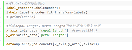
#Encode labels
label_encoder=LabelEncoder()
labels=label_encoder.fit_transform(labels)
# print(labels)
#The two-dimensional features of sepal length and petal length are selected as the clustering basis
x_axis=iris_data['sepal length'] #series(150,)
y_axis=iris_data['petal length']
data=np.array(pd.concat([x_axis,y_axis],axis=1))
gmm = GMM_EM(3)
pre_label = gmm.fit_predict(data)
print(pre_label)
print(labels)
#Cluster center obtained by Gaussian mixture algorithm
num_0,num_1,num_2=[0,0,0]
xsum_0,xsum_1,xsum_2=[0,0,0]
ysum_0,ysum_1,ysum_2=[0,0,0]
for i in range(len(pre_label)):
if pre_label[i]==0:
num_0+=1
xsum_0+=x_axis[i]
ysum_0 += y_axis[i]
elif pre_label[i]==1:
num_1+=1
xsum_1+=x_axis[i]
ysum_1 += y_axis[i]
else:
num_2+=1
xsum_2+=x_axis[i]
ysum_2 += y_axis[i]
x_center_0=xsum_0/num_0
y_center_0=ysum_0/num_0
x_center_1=xsum_1/num_1
y_center_1=ysum_1/num_1
x_center_2=xsum_2/num_2
y_center_2=ysum_2/num_2
x_center=[x_center_0,x_center_1,x_center_2]
y_center=[y_center_0,y_center_1,y_center_2]
#Actual center of dataset
x_ac_center=[x_axis[0:50].mean(),x_axis[50:100].mean(),x_axis[100:150].mean()]
y_ac_center=[y_axis[0:50].mean(),y_axis[50:100].mean(),y_axis[100:150].mean()]
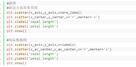
#Drawing
#Draw mixed Gaussian clustering diagram
plt.scatter(x_axis,y_axis,c=pre_label)
plt.scatter(x_center,y_center,c='r',marker='x')
plt.xlabel('sepal length')
plt.ylabel('petal length')
plt.show()
#Actual data chart
plt.scatter(x_axis,y_axis,c=labels)
plt.scatter(x_ac_center,y_ac_center,c='r',marker='x')
plt.xlabel('sepal length')
plt.ylabel('petal length')
plt.show()
# EM algorithm is sensitive to the initial value. Modifying the initial value will find that the performance of the model changes greatly
#Calculation accuracy
#Calculate the three category combinations 0 1 2 1 0 2 0 2 1 1 2 0 2 1 0 2 0 2 0 2 0 1
y_pred_1=np.array(np.zeros(150))
y_pred_2=np.array(np.zeros(150))
y_pred_3=np.array(np.zeros(150))
y_pred_4=np.array(np.zeros(150))
y_pred_5=np.array(np.zeros(150))
y_pred_6=np.array(np.zeros(150))
for i in range(150):
if pre_label[i]==0:
y_pred_1[i]=0
y_pred_2[i] = 1
y_pred_3[i] = 0
y_pred_4[i] = 1
y_pred_5[i] = 2
y_pred_6[i] = 2
if pre_label[i]==1:
y_pred_1[i] = 1
y_pred_2[i] = 0
y_pred_3[i] = 2
y_pred_4[i] = 2
y_pred_5[i] = 1
y_pred_6[i] = 0
if pre_label[i]==2:
y_pred_1[i] = 2
y_pred_2[i] = 2
y_pred_3[i] = 1
y_pred_4[i] = 0
y_pred_5[i] = 0
y_pred_6[i] = 1
def correct_rate(lei_list):
correct_num = 0
for i in range(150):
if (lei_list[i] == labels[i]):
correct_num += 1
rate = correct_num / 150
return rate
rate1=correct_rate(y_pred_1)
rate2=correct_rate(y_pred_2)
rate3=correct_rate(y_pred_3)
rate4=correct_rate(y_pred_4)
rate5=correct_rate(y_pred_5)
rate6=correct_rate(y_pred_6)
#compare
rate=[rate1,rate2,rate3,rate4,rate5,rate6]
max_rate=0
for i in range(6):
if rate[i]>max_rate:
max_rate=rate[i]
print('The accuracy is:',max_rate)