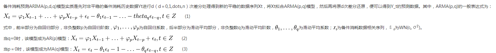
Basic concepts
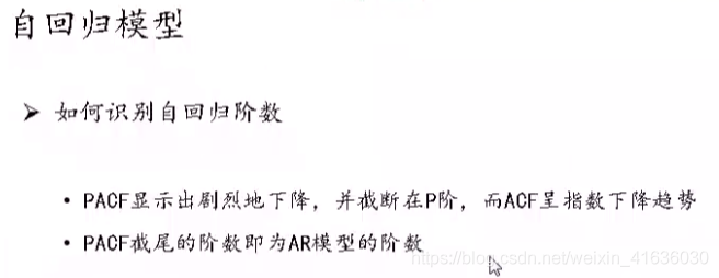
p: Autoregressive order
q: Moving average order
d: The number of differences made when the time series becomes stationary
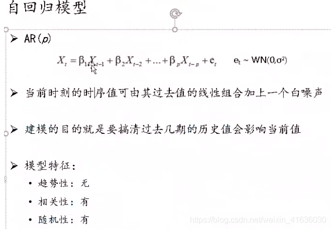
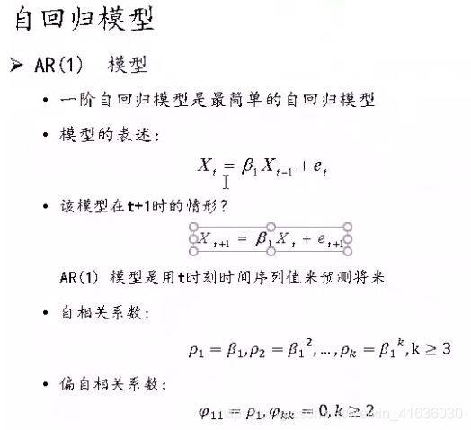
AR - Auto Regression model: AR can solve the relationship between current data and later data; Expressed as autoregressive model AR (P)
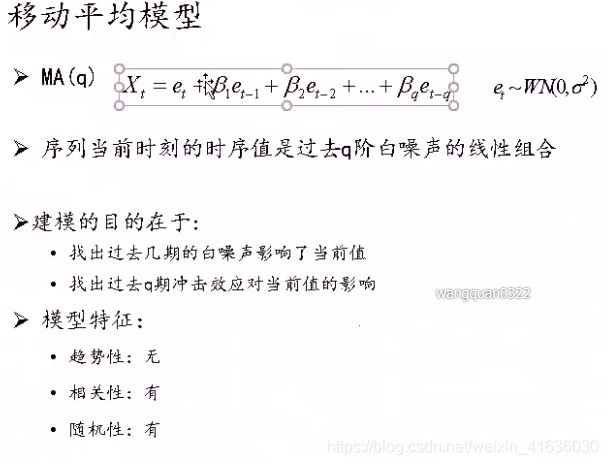
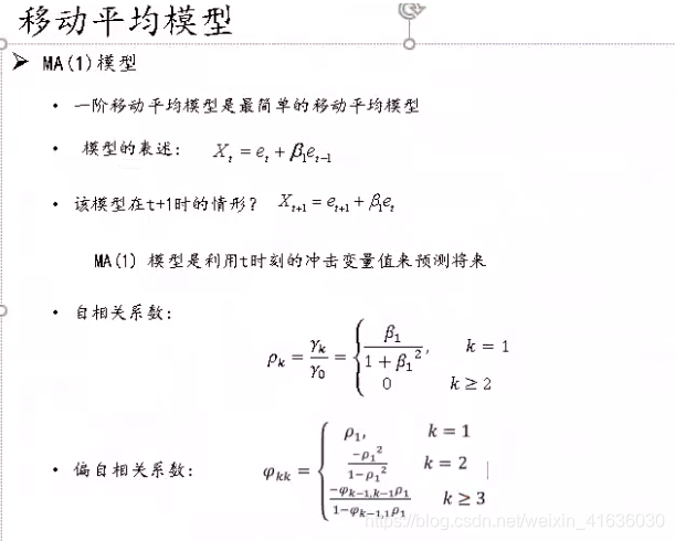
MA - Moving Average, moving average model: Ma can solve the problem of random variation, that is, noise; Expressed as moving average model MA(q)
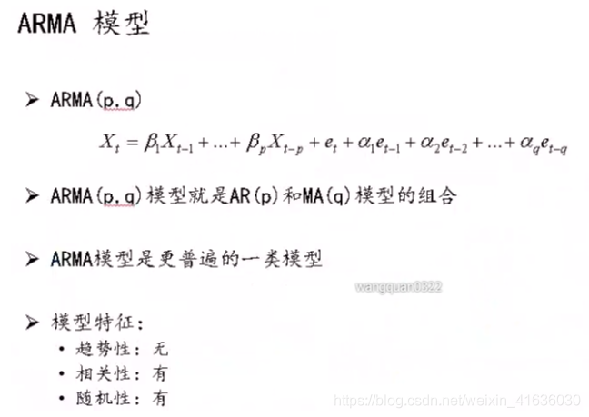
ARMA - Auto Regression and Moving Average. Autoregressive moving average model (ARMA) is composed of autoregressive (AR) and moving average model (MA); Expressed as ARMA(p, d). (the above three models can be directly applied to stationary time series models)
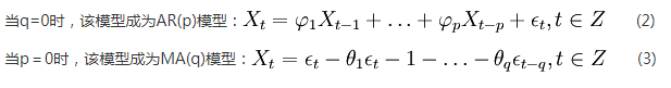
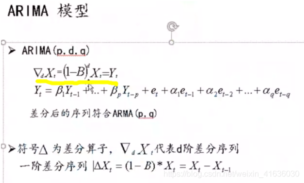
Arima - Auto Regression integral moving average, differential autoregressive moving average model. Like the previous three models, ARIMA model is also based on stable time series or stable after differential differentiation. In addition, the previous models can be regarded as a special form of ARIMA. Expressed as ARIMA(p, d, q). (for the first three models, d=0, that is, the stationary time series model does not need difference)
ARIMA model evolved from ARMA model. In fact, it makes a difference on the data before using ARMA model; In other words, ARIMA model first makes the non-stationary data stationary (using difference), and then uses ARMA model to process the stationary data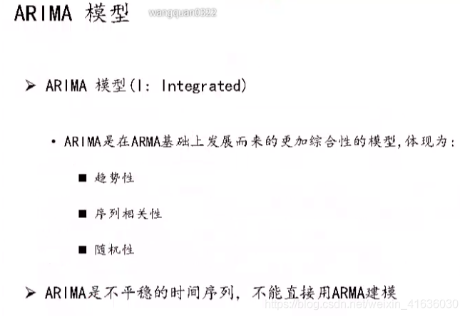
Basic process
Import model
import sys
import os
import warnings
warnings.filterwarnings("ignore")
import pandas as pd
import numpy as np
from arch.unitroot import ADF
import matplotlib.pylab as plt
%matplotlib inline
from matplotlib.pylab import style
style.use('ggplot')
import statsmodels.api as sm
import statsmodels.formula.api as smf
import statsmodels.tsa.api as smt
from statsmodels.tsa.stattools import adfuller
from statsmodels.stats.diagnostic import acorr_ljungbox
from statsmodels.graphics.api import qqplot
pd.set_option('display.float_format', lambda x: '%.5f' % x)
np.set_printoptions(precision=5, suppress=True)
"""Chinese display problem"""
plt.rcParams['font.family'] = ['sans-serif']
plt.rcParams['font.sans-serif'] = ['SimHei']
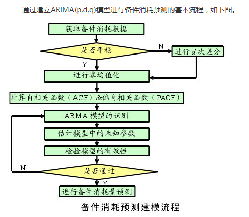
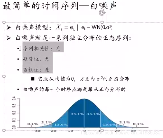
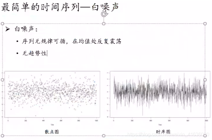
AR, MA and ARMA models must be "stationary non white noise series", so "stationarity test" and "white noise test" are required
1. Stability test
1) What is sequence stationarity
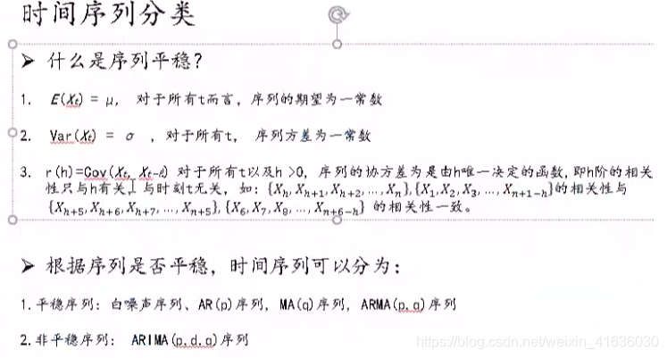
2) Check whether it is stable
The first and second methods are intuitive, but also subjective. They all rely on the judgment of the naked eye and the experience of judging people. Different people are likely to give different judgments when they see the same figure.
In most cases, the third method is selected: unit root test
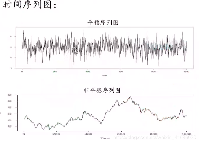
Method 1: observe the sequence diagram: if the individual value should fluctuate up and down around the mean value of the sequence, and there is no obvious upward or downward trend, it is a stable sequence.
If there is an upward or downward trend, the original sequence needs to be processed by differential stabilization. In 3) the part from unstable sequence to stationary sequence, we will talk about how to do differential stabilization
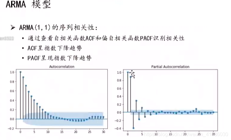
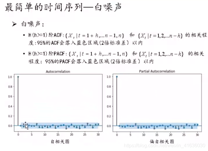
Method 2: observe the autocorrelation graph: the autocorrelation graph (ACF) and partial correlation graph (PACF) of stationary series are either tailed or truncated.
Trailing: there is always a non-zero value, which will not be equal to zero (or fluctuate randomly around 0) after k is greater than a certain constant. As the name suggests, the sequence decays slowly, and the "tail" slides down slowly
Truncation: when it is greater than a certain constant K, it quickly tends to 0 to k-order truncation, which is suddenly truncated, like a cliff
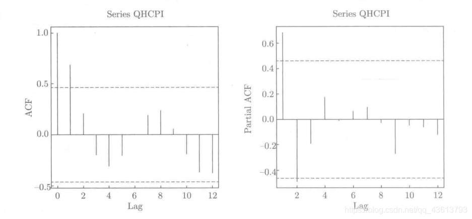
It can be seen from this figure that the left figure (autocorrelation function diagram) shows the tailing feature (second-order tailing), while the right figure (partial autocorrelation function diagram) shows the tailing feature (second-order tailing)
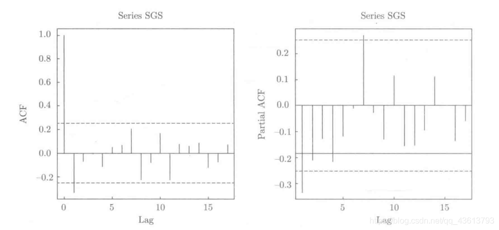
As can be seen from this figure, the left figure (autocorrelation function diagram) shows the truncated feature (first-order truncated), while the right figure (partial autocorrelation function diagram) shows the tailed feature (first-order tailed)
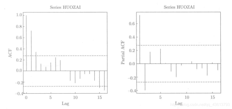
It can be seen from this figure that the left figure (autocorrelation function diagram) shows the tailing feature (second-order tailing), and the right figure (partial autocorrelation function diagram) also shows the tailing feature (first-order tailing)
Method 3: unit root test: when there is a unit root in the polynomial equation of the lag operator of a time series, we believe that the time series is non-stationary; On the contrary, when the equation has no unit root, we think the time series is stable.
Common unit root test methods include DF test, ADF test and PP test. Today we will use ADF test to demonstrate for you
In Python, two commonly used packages provide ADF verification, statsmodel and arch.
The first method is to use statsmodel:
from statsmodels.stats.diagnostic import unitroot_adf

unitroot_adf(df.pct_chg)
Output is:
The test value p-value,Lag order, degree of freedom and other information.
We see that the test statistic is-14.46,Much less than 1%Critical value of-3.47,Namely p The value is much less than 0.01,Therefore, we reject the original hypothesis and think that the time series is stable. (the original assumption here is that there is a unit root, that is, the time series is non-stationary.)
The second method: using arch is:
from arch.unitroot import ADF

ADF(df.pct_chg)
Its output information is basically consistent with statsmodel.
or
Use method II for other cases
print("Unit root test:\n")
print(ADF(data.diff1.dropna()))
Unit root test:

   Augmented Dickey-Fuller Results
=====================================
Test Statistic                 -3.156
P-value                         0.023
Lags                                0
-------------------------------------

Trend: Constant
Critical Values: -3.63 (1%), -2.95 (5%), -2.61 (10%)
Null Hypothesis: The process contains a unit root.
Alternative Hypothesis: The process is weakly stationary.
Unit root test: the unit root test is conducted on the first-order difference, and the comparison between the statistical value of 1%,% 5,% 10 rejecting the original hypothesis and the ADF Test result is obtained. In this data, the P-value is 0.023, close to 0, and the ADF Test result is less than 5% and 10% at the same time, which indicates that the hypothesis is well rejected. In this data, the ADF result is -3.156, rejecting the original hypothesis, That is, the data is stable after the first-order difference.
Method 4: the above methods are integrated, that is, the results are more convincing
1. Draw a sequence diagram and observe whether there is fluctuation and upward or downward trend
2. Make the correlation coefficient diagram. If the autocorrelation coefficient decays rapidly with the increase of time interval k, the sequence is stable; If the autocorrelation coefficient decays slowly with the increase of time interval k, the sequence is unstable
3. Carry out unit root test, P-value< α The original assumption that there is a unit root is rejected and the sequence is stable.
3) From unstable sequence to stationary sequence
Taking logarithm can eliminate the trend of data fluctuation
The difference of series can eliminate the trend and seasonality of data growth.
For non-stationary series, if the result after difference does not meet the requirements, it is necessary to continue the difference on the original basis until the result after difference belongs to stationary series
Methods: differential transformation
fig = plt.figure(figsize=(12,8))
ax1= fig.add_subplot(111)
diff1 = dta.diff(1)
diff1.plot(ax=ax1)
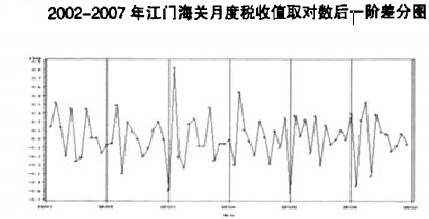
As can be seen from the figure below, the figure after the logarithm of the prediction sequence is taken and the first-order difference is made
Select one of the inspection methods and find:
The graphical display after the logarithm of the prediction series and the first-order difference basically eliminates the influence of long-term trend, tends to be stable, and meets the basic requirements of ARIMA model modeling.
2. White noise inspection
from statsmodels.stats.diagnostic import acorr_ljungbox
acorr_ljungbox(data.diff1.dropna(), lags = [i for i in range(1,12)],boxpierce=True)
(array([11.30402, 13.03896, 13.37637, 14.24184, 14.6937 , 15.33042,
        16.36099, 16.76433, 18.15565, 18.16275, 18.21663]),
 array([0.00077, 0.00147, 0.00389, 0.00656, 0.01175, 0.01784, 0.02202,
        0.03266, 0.03341, 0.05228, 0.07669]),
 array([10.4116 , 11.96391, 12.25693, 12.98574, 13.35437, 13.85704,
        14.64353, 14.94072, 15.92929, 15.93415, 15.9696 ]),
 array([0.00125, 0.00252, 0.00655, 0.01135, 0.02027, 0.03127, 0.04085,
        0.06031, 0.06837, 0.10153, 0.14226]))
Pass p< α, The original assumption is rejected, so the sequence after difference is a stable non white noise sequence, which can be modeled in the next step
3. Model order determination: calculate the autocorrelation function ACF and partial autocorrelation function PACF
If you choose method 2 as the test method, you have obtained ACF and PACF, but the best test method is unit root test
technological process:
1. According to the ACF diagram and PACF diagram, which model of AR, MA and ARMA is used after the sequence is stabilized
2. Judge the order of p and q
(the first two steps are based on ACF and PACF diagrams)
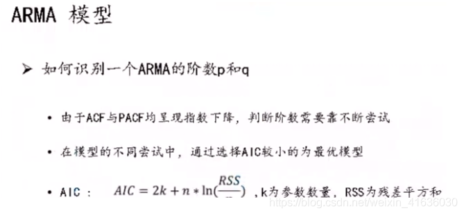
3. ARMA may have multiple models determined by p and q (because multiple p and q can be seen in ACF and PACF diagrams). At this time, it is necessary to assist in selecting models through information standards AIC and BIC
Choose the one with the lowest AIC and BIC values, because the smaller the AIC and BIC, the better the model
However, it should be noted that these criteria can not explain the accuracy of a certain model, that is, for the three models a, B and C, we can judge that model C is the best, but we can not guarantee that model C can depict the data well, because it is possible that all three models are bad.
Akaike information criterion: AIC encourages the goodness of data fitting, but tries to avoid overfitting. Therefore, the preferred model should be the one with the lowest AIC value

Bayesian information criterion:

Where L is the maximum likelihood under the model, n is the number of data, and k is the number of variables of the model.
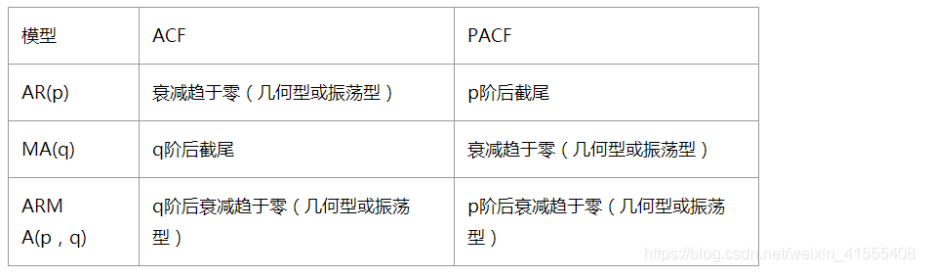
| Model | ACF | PACF |
|---|---|---|
| AR | Trailing | Truncation |
| MA | Truncation | Trailing |
| ARMA | Trailing | Trailing |
Check the autocorrelation diagram and partial autocorrelation diagram of stationary time series.
Through SM graphics. tsa. plot_ ACF and SM graphics. tsa. plot_ PACF get graphics
Where lags represents the order of lag. ACF diagram and PACF diagram are obtained respectively
Example 1:
1) Observe the ACF and PACF diagrams to determine which model it is
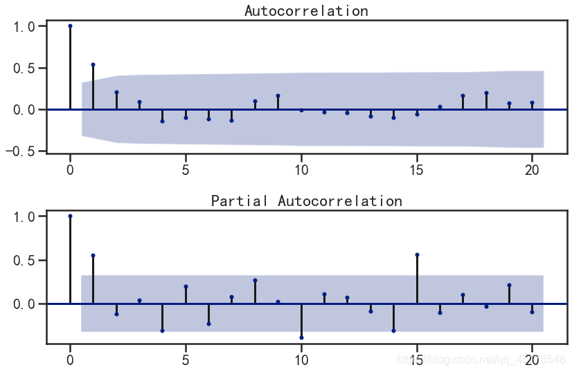
dta= dta.diff(1)#We already know that we need to use the time series of first-order difference, and the previous procedure for judging the difference can be commented out
fig = plt.figure(figsize=(12,8))
ax1=fig.add_subplot(211)
fig = sm.graphics.tsa.plot_acf(dta,lags=40,ax=ax1)
ax2 = fig.add_subplot(212)
fig = sm.graphics.tsa.plot_pacf(dta,lags=40,ax=ax2)
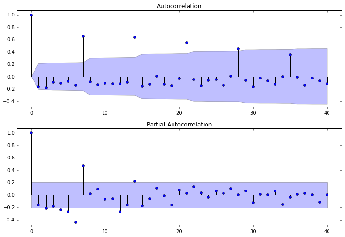
It can be observed from two figures:
- The autocorrelation diagram shows that the lag has three orders beyond the confidence boundary;
- The partial correlation diagram shows that the partial autocorrelation coefficient exceeds the confidence boundary when it lags 1 to 7 orders (lags 1,2,..., 7). If the partial autocorrelation coefficient is reduced to 0 after lag 7, the following models can be selected:
- ARMA(0,1) model: that is, the autocorrelation graph is reduced to 0 after lagging 1 order, and the partial autocorrelation is reduced to 0, which is a moving average model with order q=1;
- ARMA(7,0) model: that is, the partial autocorrelation graph is reduced to 0 after lagging 7 orders, and the autocorrelation is reduced to 0, which is an autoregressive model with level p=3;
- ARMA(7,1) model: even if the autocorrelation and partial autocorrelation are reduced to zero. Is a hybrid model.
2) AIC BIC selects the best model
dta is a differential sequence
Because the ARMA model is used
arma_mod20 = sm.tsa.ARMA(dta,(7,0)).fit() # dta is a differential sequence
print(arma_mod20.aic,arma_mod20.bic,arma_mod20.hqic)
arma_mod30 = sm.tsa.ARMA(dta,(0,1)).fit()
print(arma_mod30.aic,arma_mod30.bic,arma_mod30.hqic)
arma_mod40 = sm.tsa.ARMA(dta,(7,1)).fit()
print(arma_mod40.aic,arma_mod40.bic,arma_mod40.hqic)
arma_mod50 = sm.tsa.ARMA(dta,(8,0)).fit()
print(arma_mod50.aic,arma_mod50.bic,arma_mod50.hqic)

It can be seen that ARMA(7,0) has the smallest AIC, BIC and HQIC, so it is the best model.
Example 2:
1) What kind of observation and judgment model is ACF
From the autocorrelation diagram and partial autocorrelation diagram of the first-order difference sequence, it can be found that:
- Autocorrelation graph tailing or first-order truncation
- First order truncation of partial autocorrelation graph,
- Therefore, we can establish ARIMA(1,1,0), ARIMA(1,1,1) and ARIMA(0,1,1) models.
2) AIC BIC selects the best model
data ["xt"] is a sequence without difference
Because ARIMA model is used
arma_mod20 = sm.tsa.ARIMA(data["xt"],(1,1,0)).fit() # data["xt"] is data without difference
arma_mod30 = sm.tsa.ARIMA(data["xt"],(0,1,1)).fit()
arma_mod40 = sm.tsa.ARIMA(data["xt"],(1,1,1)).fit()
values = [[arma_mod20.aic,arma_mod20.bic,arma_mod20.hqic],[arma_mod30.aic,arma_mod30.bic,arma_mod30.hqic],[arma_mod40.aic,arma_mod40.bic,arma_mod40.hqic]]
df = pd.DataFrame(values,index=["AR(1,1,0)","MA(0,1,1)","ARMA(1,1,1)"],columns=["AIC","BIC","hqic"])
df
| AIC | BIC | hqic | |
|---|---|---|---|
| AR(1,1,0) | 253.09159 | 257.84215 | 254.74966 |
| MA(0,1,1) | 251.97340 | 256.72396 | 253.63147 |
| ARMA(1,1,1) | 254.09159 | 258.84535 | 259.74966 |
Select model MA(0, 1, 1), namely ARIMA(0, 1, 1)
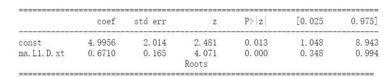
4. Parameter estimation
from statsmodels.tsa.arima_model import ARIMA
model = ARIMA(data["xt"], order=(0,1,1))
result = model.fit()
print(result.summary())
                             ARIMA Model Results
==============================================================================
Dep. Variable:                   D.xt   No. Observations:                   36
Model:                 ARIMA(0, 1, 1)   Log Likelihood                -122.987
Method:                       css-mle   S.D. of innovations              7.309
Date:                Tue, 22 Dec 2020   AIC                            251.973
Time:                        09:11:55   BIC                            256.724
Sample:                    01-01-1953   HQIC                           253.631
                         - 01-01-1988
==============================================================================
                 coef    std err          z      P>|z|      [0.025      0.975]
------------------------------------------------------------------------------
const          4.9956      2.014      2.481      0.013       1.048       8.943
ma.L1.D.xt     0.6710      0.165      4.071      0.000       0.348       0.994
                                    Roots
=============================================================================
                  Real          Imaginary           Modulus         Frequency
-----------------------------------------------------------------------------
MA.1           -1.4902           +0.0000j            1.4902            0.5000
-----------------------------------------------------------------------------
5. Model test

1) Significance test of parameters

P< α, Rejecting the original hypothesis, it is considered that the parameter is significantly non-zero, and the MA(2) model fits the sequence, and the residual sequence has realized white noise
2) Significance test of model

resid = result.resid#residual
fig = plt.figure(figsize=(12,8))
ax = fig.add_subplot(111)
fig = qqplot(resid, line='q', ax=ax, fit=True)
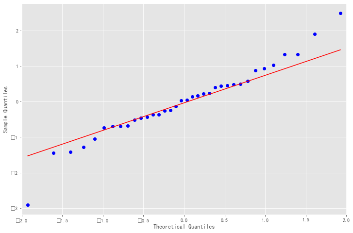
As shown in the qq chart, we can see that the red KDE line is parallel to N(0,1), which is a good indicator of the positive distribution of residues. It shows that the residual sequence is a white noise sequence, and the information of the model is fully extracted. When you can also use the LB statistic introduced earlier to test the white noise
ARIMA(0,1,1) model fits the sequence, the residual sequence has realized white noise, and the parameters are significantly non-zero. It shows that ARIMA(0,1,1) model is an effective fitting model of the sequence
6. Model prediction
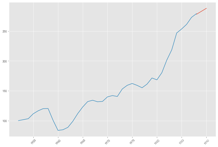
pred = result.predict('1988', '1990',dynamic=True, typ='levels')
print (pred)
1988-01-01   278.35527
1989-01-01   283.35088
1990-01-01   288.34649
Freq: AS-JAN, dtype: float64
plt.figure(figsize=(12, 8))
plt.xticks(rotation=45)
plt.plot(pred)
plt.plot(data.xt)
plt.show()
7. Analysis of prediction results
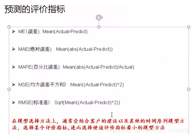
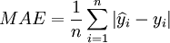
Mean absolute error:
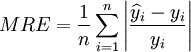
Average relative error:
Predicted mean square deviation:
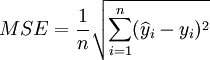
Where, y_i is the actual data of the sequence, Forecast data for the model.
For example:
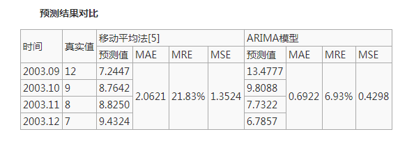
From the comparison of the prediction results and various evaluation indexes in the above table, the prediction results of ARIMA model are significantly better than the moving average method. From the perspective of average relative error, ARIMA model is 6.93%, which is nearly 15% higher than the moving average method, and the mean square deviation of prediction is also small, only 0.4298. It can be seen that the model can accurately predict the change trend of spare parts consumption and provide a basis for the prediction of spare parts consumption.
quote:
https://blog.csdn.net/qixizhuang/article/details/86716149
https://zhidao.baidu.com/question/288273884.html
https://zhuanlan.zhihu.com/p/343617191
https://blog.csdn.net/qq_43613793/article/details/109908418
https://blog.csdn.net/qq_45176548/article/details/116771331
https://blog.csdn.net/weixin_41555408/article/details/117218457
https://blog.csdn.net/weixin_41636030/article/details/89138638
https://www.zhihu.com/question/48447779/answer/112330897
https://blog.csdn.net/u010414589/article/details/49622625
https://wiki.mbalib.com/wiki/ARIMA%E6%A8%A1%E5%9E%8B
https://blog.csdn.net/qq_45176548/article/details/111504846