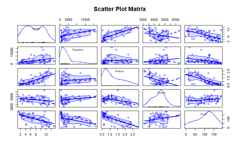
The data is still state Take x77 data set as an example to explore the relationship between a state's crime rate and other factors, including population, illiteracy rate, average income and frost days (the average days when the temperature is below freezing).
Label explanation: Murder crime rate, Population, Illiteracy illiteracy rate, Income income Income, Frost frosting days
The multiple linear regression of interactive items mainly uses the vehicle data in mtcars data, takes the vehicle weight and horsepower as the prediction variables, and includes interactive items to fit the regression model.
Among them, hp vehicle power and wt vehicle weight.
Experimental process:
1. Analyze the relationship between two variables
It can be seen that the relationship between illiteracy rate and crime rate is relatively large, reaching about 70%.
scatterplotMatrix() function draws the scatter plot on the non diagonal line, and adds smooth and linear fitting curves. The diagonal line is to draw the density map and whisker map of each variable.
The murder rate is a bimodal curve, and there is a deviation in each prediction variable. Look at the data in the first row of the murder rate. From the fitting effect, the murder rate increases with the increase of population and illiteracy rate, and decreases with the decrease of income level and frosting days.
Look at the last graph in the last row. The last graph is the frosting days. The curve is the fitting effect of frosting days. The vertical axis is the frosting days. Other graphs are the changes of variables under the influence of frosting days. It can be seen that the colder it is, the lower the illiteracy rate will be, and the higher the income will be
2. Multiple linear regression
When the prediction variable is not 1, the regression coefficient indicates the number of dependent variables to be increased when one prediction variable is increased by one unit and other prediction variables remain unchanged.
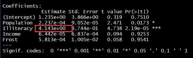
① LM (murder ~ population + intelligence + income + frost, data = States) function fitting multiple linear regression
② In this experiment, it can be seen from the results that the regression coefficient of the illiteracy rate is 4.14 (Note: 4.134e+00=4.134x10^0). Therefore, under the control of population, income and temperature, if the illiteracy rate increases by 1%, the murder rate will increase by 4.14%. Its coefficient is significantly non-zero at the level of P < 0.001.
Look at Forst, the regression coefficient is 0.00058. Similarly, it is not significant, not 0, so it is not linear.
Note:
An asterisk corresponds to the significance level of 5%, that is, P < 0.05, P < 0.05 indicates that there is at least 95% confidence in the occurrence of something.
The two asterisks correspond to a significant level of 1%, i.e. P < 0.01, P < 0.01, indicating that there is at least 99% confidence in the occurrence of something.
The three asterisks correspond to a significant level of 0.1%, that is, P < 0.001. P < 0.001 indicates that there is at least 99.9% confidence in the occurrence of something.
The more asterisks, the smaller the p value, the stronger the significance.
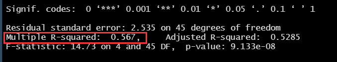
The predictive variables can explain the variance of 57% of the murder rate in each state.
3. Multiple linear regression of significant interaction items (automobile data set)
It is mainly explored from PR (> |t|)
From the perspective of Pr, the interaction term between power and vehicle weight is significant, which means that the relationship between the response variable and one of the prediction variables depends on the level of the other prediction variable. Again, it means that the relationship between miles per gallon of gasoline and vehicle power varies with vehicle weight.
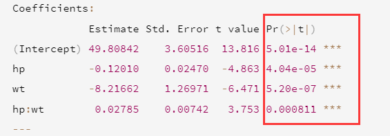
The prediction model mpg is mpg=49.81 - 0.12 x hp - 8.22 x wt + 0.03 x hp x wt
Use wt=3.2, less than one standard deviation or more than one, that is, wt=4.2 and wt=2.2.
When substituting wt separately, you will find that the expected change of mpg is decreasing. The effect function in the effects package is shown in detail as follows.
It is clear that the relationship between power and miles per gallon decreases with the increase of vehicle weight. When wt=4.2, the straight line is almost horizontal, indicating that hp increases and mpg will not change.

> #Detect the correlation of each variable
> states <- as.data.frame(state.x77[,c("Murder","Population","Illiteracy","Income","Frost")])

> cor(states)
               Murder Population Illiteracy     Income      Frost
Murder      1.0000000  0.3436428  0.7029752 -0.2300776 -0.5388834
Population  0.3436428  1.0000000  0.1076224  0.2082276 -0.3321525
Illiteracy  0.7029752  0.1076224  1.0000000 -0.4370752 -0.6719470
Income     -0.2300776  0.2082276 -0.4370752  1.0000000  0.2262822
Frost      -0.5388834 -0.3321525 -0.6719470  0.2262822  1.0000000

> #Detect bivariate relationship
> library(car)

> scatterplotMatrix(states,spread=FALSE,smooth.args=list(lty=2),main="Scatter Plot Matrix")

> #multiple linear regression
> fit <- lm(Murder ~ Population + Illiteracy + Income + Frost,data=states)

> summary(fit)

Call:
lm(formula = Murder ~ Population + Illiteracy + Income + Frost,
    data = states)

Residuals:
    Min      1Q  Median      3Q     Max
-4.7960 -1.6495 -0.0811  1.4815  7.6210

Coefficients:
             Estimate Std. Error t value Pr(>|t|)
(Intercept) 1.235e+00  3.866e+00   0.319   0.7510
Population  2.237e-04  9.052e-05   2.471   0.0173 *
Illiteracy  4.143e+00  8.744e-01   4.738 2.19e-05 ***
Income      6.442e-05  6.837e-04   0.094   0.9253
Frost       5.813e-04  1.005e-02   0.058   0.9541
---
Signif. codes:  0 '***' 0.001 '**' 0.01 '*' 0.05 '.' 0.1 ' ' 1

Residual standard error: 2.535 on 45 degrees of freedom
Multiple R-squared:  0.567,	Adjusted R-squared:  0.5285
F-statistic: 14.73 on 4 and 45 DF,  p-value: 9.133e-08


> #Multiple linear regression with significant interaction terms
> fit1 <- lm(mpg ~ hp + wt + hp:wt,data = mtcars)

> summary(fit1)

Call:
lm(formula = mpg ~ hp + wt + hp:wt, data = mtcars)

Residuals:
    Min      1Q  Median      3Q     Max
-3.0632 -1.6491 -0.7362  1.4211  4.5513

Coefficients:
            Estimate Std. Error t value Pr(>|t|)
(Intercept) 49.80842    3.60516  13.816 5.01e-14 ***
hp          -0.12010    0.02470  -4.863 4.04e-05 ***
wt          -8.21662    1.26971  -6.471 5.20e-07 ***
hp:wt        0.02785    0.00742   3.753 0.000811 ***
---
Signif. codes:  0 '***' 0.001 '**' 0.01 '*' 0.05 '.' 0.1 ' ' 1

Residual standard error: 2.153 on 28 degrees of freedom
Multiple R-squared:  0.8848,	Adjusted R-squared:  0.8724
F-statistic: 71.66 on 3 and 28 DF,  p-value: 2.981e-13


> library(statmod)

> library(carData)

> library(effects)

> plot(effect("hp:wt",fit1,,list(wt=c(2.2,3.2,4.2))),multiline=TRUE)
There were 50 or more warnings (use warnings() to see the first 50)