Basic information of the paper

• Title: HybridSN: Exploring 3-D – 2-DCNN Feature Hierarchy for Hyperspectral Image Classification
• Author: swalpa Kumar Roy, student member, IEEE, gopal Krishna, SHIV ram Dubey, member, IEEE, and bidyut B. Chaudhuri, life fellow, IEEE
• Time: 2019
• Paper address: arXiv:1902.06701v3 [cs.CV] 3 Jul 2019
• code: https://github.com/OUCTheoryGroup/colab_demo/blob/master/202003_models/HybridSN_GRSL2020.ipynb

Research background

Hyperspectral image classification is widely used in the analysis of remote sensing images. Hyperspectral images include images of different bands. Convolutional neural network (CNN) is a common visual data processing method based on deep learning. The use of CNN for HSI classification can also be seen in recent articles. Most of these methods are based on 2D CNN. However, HSI classification performance is highly dependent on spatial and spectral information. Due to the increase of computational complexity, there are few methods to use 3D CNN. In this paper, a hybrid spectral convolutional neural network (HybridSN) for HSI classification is proposed. Basically, HybridSN is a spectral spatial 3D-CNN, followed by spatial 2D-CNN. 3D-CNN promotes the joint spatial spectral feature representation from the spectral band stack. 2D-CNN on top of 3D-CNN further learns more abstract hierarchical space representation. In addition, using hybrid CNN reduces the complexity of the model than using 3D-CNN alone.

Questions after reading the summary

• What is hyperspectral?
• Model structure of HybridSN

Answers to the above questions after reading the article

Hyperspectral Fundamentals

• Monochromatic light: light of a single wavelength (or frequency) that cannot produce dispersion.
• Polychromatic light: light synthesized by several monochromatic lights.
• Dispersion system: the phenomenon that polychromatic light is decomposed into monochromatic light to form a spectrum.
• Spectrum (optical spectrum): a pattern in which the monochromatic light dispersed is sequentially arranged according to the wavelength (or frequency) after the dichroic light is divided by the dispersion system (such as prism and grating).
• Grating: an optical device consisting of a large number of parallel slits of equal width and equal spacing.
• Hyperspectral Image: detailed segmentation is carried out in the spectral dimension, which is not only the difference between traditional black, white or RGB, but also N channels in the spectral dimension. For example, we can divide 400nm-1000nm into 300 channels. Once, a data cube is obtained through hyperspectral equipment, which not only has the information of the image, but also expands it in the spectral dimension. As a result, we can not only obtain the spectral data of each point on the image, but also obtain the image information of any spectral segment.
• Imaging principle of hyperspectral image: after the one-dimensional information in space passes through the lens and slit, light of different wavelengths propagates according to different degrees of dispersion. Each point on the one-dimensional image is diffracted and divided through the grating to form a spectral band, which irradiates on the detector. The position and intensity of each pixel on the detector characterize the spectrum and intensity.
• H SI: digital image model, which reflects the way people'S visual system perceives color. It perceives color with three basic feature quantities: Hue (Hue), Saturation (Saturation) and brightness I (Intensity).
• Hue H (hue): it is related to the frequency of light wave. It represents the feeling of human senses on different colors, and can also represent a certain range of colors;
• Saturation S: indicates the purity of the color. The pure spectral color is completely saturated. Adding white light will dilute the saturation. The greater the saturation, the brighter the color looks.
• Brightness I (Intensity): corresponds to the imaging brightness and image gray level. It is the brightness of the color.

HybridSN

According to the above description, 2D CNN is difficult to fully extract hyperspectral spatial information, while 3D CNN is rarely used due to the huge amount of computation.
In this paper, 2D and 3D CNN are combined, 3D CNN is used to extract hyperspectral spatial features, and 2D CNN is used for more abstract hierarchical spatial representation.

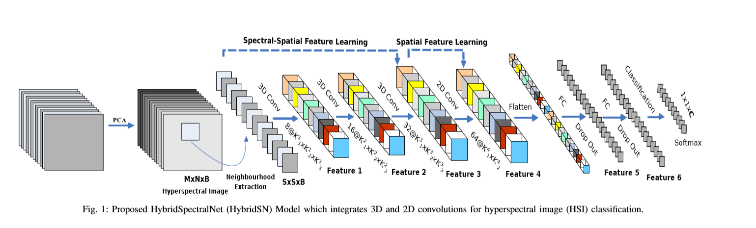
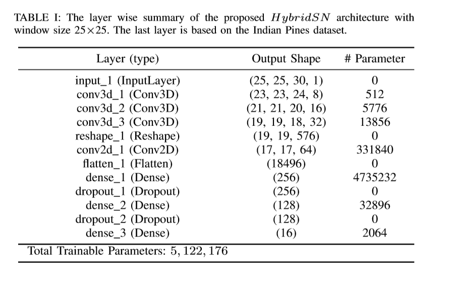
The network structure is shown in the figure above (3 three-dimensional convolutions, 1 two-dimensional convolution, 3 full connection layers):

• In three-dimensional convolution, the size of convolution kernel is 8 × three × three × seven × 1,16 × three × three × five × 8,32 × three × three × three × 16 (16 3D cores, 3) × three × (5d)
• In two-dimensional convolution, the size of convolution kernel is 64 × three × three × 576 (576 is the number of two-dimensional input feature maps)
  

experimental verification

Dataset description

Three open source hyperspectral image datasets, Indian Pines (IP), University of Pavia (UP) and Salinas Scene (SA)

IP image space dimension: 145 × 145, with a wavelength range of 400-2500 nm and a total of 224 spectral bands
UP image space dimension: 610 × 340, wavelength range 430-860nm, a total of 103 spectral bands
SA image space dimension: 512 × 217, with a wavelength range of 360-2500 nm and a total of 224 spectral bands

Classification results

Overall Accuracy (OA), Average Accuracy (AA) and Kappa Coefficient (Kappa) were used to judge the classification performance of HSI. Where OA represents the number of correctly classified samples in the overall test samples; AA represents the average value of classification accuracy; Kappa is a measure of statistical measurement, which provides mutual information about the strong consistency between ground truth map and classification map. The results of the proposed HybridSN model are compared with the most widely used monitoring methods such as SVM[33], 2D-CNN[34], 3D-CNN[35], M3D-CNN[36] and SSRN[27]. 30% and 70% of the data were randomly divided into training group and test group 2. We used the public code 3 of the comparison method to calculate the result.



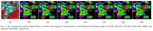
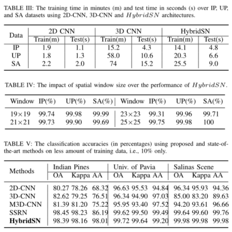
It can be seen from table 2 that the hybrid algorithm is superior to all comparison methods in each data set while maintaining the minimum standard deviation.
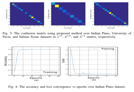
Figure 3 shows the confusion matrix of HSI classification performance of hybrid networks on IP, UP and SA data sets.
The accuracy and loss convergence of 100 epochs in the training set and verification set are shown in Figure 4. It can be seen that the convergence time is about 50 epochs, which shows that the convergence speed of the author's method is fast.
The calculation efficiency of hybrid network model is reflected in the number of training and testing, as shown in Table 3.

code analysis

Three dimensional convolution part:
conv1: (1, 30, 25, 25), 8 convolution kernels of 7x3x3 = = > (8, 24, 23, 23)
conv2: (8, 24, 23, 23), 16 5x3x3 convolution kernels = = > (16, 20, 21, 21)
conv3: (16, 20, 21, 21), 32 convolution kernels of 3x3x3 = = > (32, 18, 19, 19)
Next, we need to carry out two-dimensional convolution, so take the previous 32*18 reshape and get (576, 19, 19)
Two dimensional convolution part:
(576, 19, 19) 64 3x3 convolution kernels are obtained (64, 17, 17)
Next is a flatten operation, which becomes a vector of 18496 dimensions,
Next is the full connection layer of 256128 nodes, all of which use Dropout with a ratio of 0.4,
The final output is 16 nodes, which is the final number of classification categories.

! wget http://www.ehu.eus/ccwintco/uploads/6/67/Indian_pines_corrected.mat
! wget http://www.ehu.eus/ccwintco/uploads/c/c4/Indian_pines_gt.mat
! pip install spectral
#Get the data and import it into the basic library
import numpy as np
import matplotlib.pyplot as plt
import scipy.io as sio
from sklearn.decomposition import PCA
from sklearn.model_selection import train_test_split
from sklearn.metrics import confusion_matrix, accuracy_score, classification_report, cohen_kappa_score
import spectral
import torch
import torchvision
import torch.nn as nn
import torch.nn.functional as F
import torch.optim as optim

Define the HybridSN class:

class_num = 16

class HybridSN(nn.Module):
  ''' your code here '''
  def __init__(self):
    super(HybridSN, self).__init__()
    self.conv3d_1 = nn.Sequential(
        nn.Conv3d(1, 8, kernel_size=(7, 3, 3), stride=1, padding=0),
        nn.BatchNorm3d(8),
        nn.ReLU(inplace = True),
    )
    self.conv3d_2 = nn.Sequential(
        nn.Conv3d(8, 16, kernel_size=(5, 3, 3), stride=1, padding=0),
        nn.BatchNorm3d(16),
        nn.ReLU(inplace = True),
    ) 
    self.conv3d_3 = nn.Sequential(
        nn.Conv3d(16, 32, kernel_size=(3, 3, 3), stride=1, padding=0),
        nn.BatchNorm3d(32),
        nn.ReLU(inplace = True)
    )

    self.conv2d_4 = nn.Sequential(
        nn.Conv2d(576, 64, kernel_size=(3, 3), stride=1, padding=0),
        nn.BatchNorm2d(64),
        nn.ReLU(inplace = True),
    )
    self.fc1 = nn.Linear(18496,256)
    self.fc2 = nn.Linear(256,128)
    self.fc3 = nn.Linear(128,16)
    self.dropout = nn.Dropout(p = 0.4)

  def forward(self,x):
    out = self.conv3d_1(x)
    out = self.conv3d_2(out)
    out = self.conv3d_3(out)
    out = self.conv2d_4(out.reshape(out.shape[0],-1,19,19))
    out = out.reshape(out.shape[0],-1)
    out = F.relu(self.dropout(self.fc1(out)))
    out = F.relu(self.dropout(self.fc2(out)))
    out = self.fc3(out)
    return out
# Random input to test whether the network structure is connected
# x = torch.randn(1, 1, 30, 25, 25)
# net = HybridSN()
# y = net(x)
# print(y.shape)

Create dataset
Firstly, PCA dimensionality reduction is applied to hyperspectral data; Then create a data format that can be easily processed by keras; Then 10% of the data are randomly selected as the training set and the rest as the test set.

First, define the basic function:

# Applying PCA transform to hyperspectral data X
def applyPCA(X, numComponents):
    newX = np.reshape(X, (-1, X.shape[2]))
    pca = PCA(n_components=numComponents, whiten=True)
    newX = pca.fit_transform(newX)
    newX = np.reshape(newX, (X.shape[0], X.shape[1], numComponents))
    return newX

# When a patch is extracted around a single pixel, the edge pixels cannot be obtained. Therefore, this part of pixels is padded
def padWithZeros(X, margin=2):
    newX = np.zeros((X.shape[0] + 2 * margin, X.shape[1] + 2* margin, X.shape[2]))
    x_offset = margin
    y_offset = margin
    newX[x_offset:X.shape[0] + x_offset, y_offset:X.shape[1] + y_offset, :] = X
    return newX

# The patch is extracted around each pixel and then created into a format consistent with keras processing
def createImageCubes(X, y, windowSize=5, removeZeroLabels = True):
    # padding X
    margin = int((windowSize - 1) / 2)
    zeroPaddedX = padWithZeros(X, margin=margin)
    # split patches
    patchesData = np.zeros((X.shape[0] * X.shape[1], windowSize, windowSize, X.shape[2]))
    patchesLabels = np.zeros((X.shape[0] * X.shape[1]))
    patchIndex = 0
    for r in range(margin, zeroPaddedX.shape[0] - margin):
        for c in range(margin, zeroPaddedX.shape[1] - margin):
            patch = zeroPaddedX[r - margin:r + margin + 1, c - margin:c + margin + 1]   
            patchesData[patchIndex, :, :, :] = patch
            patchesLabels[patchIndex] = y[r-margin, c-margin]
            patchIndex = patchIndex + 1
    if removeZeroLabels:
        patchesData = patchesData[patchesLabels>0,:,:,:]
        patchesLabels = patchesLabels[patchesLabels>0]
        patchesLabels -= 1
    return patchesData, patchesLabels

def splitTrainTestSet(X, y, testRatio, randomState=345):
    X_train, X_test, y_train, y_test = train_test_split(X, y, test_size=testRatio, random_state=randomState, stratify=y)
    return X_train, X_test, y_train, y_test

Read and create the dataset below:

# Feature category
class_num = 16
X = sio.loadmat('Indian_pines_corrected.mat')['indian_pines_corrected']
y = sio.loadmat('Indian_pines_gt.mat')['indian_pines_gt']

# Proportion of samples used for testing
test_ratio = 0.90
# The size of the extracted patch around each pixel
patch_size = 25
# PCA dimension reduction is used to obtain the number of principal components
pca_components = 30

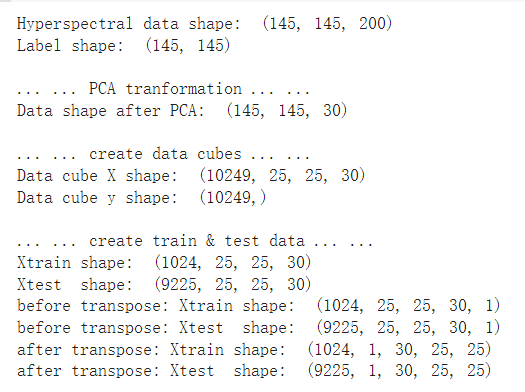
print('Hyperspectral data shape: ', X.shape)
print('Label shape: ', y.shape)

print('\n... ... PCA tranformation ... ...')
X_pca = applyPCA(X, numComponents=pca_components)
print('Data shape after PCA: ', X_pca.shape)

print('\n... ... create data cubes ... ...')
X_pca, y = createImageCubes(X_pca, y, windowSize=patch_size)
print('Data cube X shape: ', X_pca.shape)
print('Data cube y shape: ', y.shape)

print('\n... ... create train & test data ... ...')
Xtrain, Xtest, ytrain, ytest = splitTrainTestSet(X_pca, y, test_ratio)
print('Xtrain shape: ', Xtrain.shape)
print('Xtest  shape: ', Xtest.shape)

# Change the shape of xtrain and ytrain to meet the requirements of keras
Xtrain = Xtrain.reshape(-1, patch_size, patch_size, pca_components, 1)
Xtest  = Xtest.reshape(-1, patch_size, patch_size, pca_components, 1)
print('before transpose: Xtrain shape: ', Xtrain.shape) 
print('before transpose: Xtest  shape: ', Xtest.shape) 

# In order to adapt to the pytorch structure, the data should be transferred
Xtrain = Xtrain.transpose(0, 4, 3, 1, 2)
Xtest  = Xtest.transpose(0, 4, 3, 1, 2)
print('after transpose: Xtrain shape: ', Xtrain.shape) 
print('after transpose: Xtest  shape: ', Xtest.shape) 


""" Training dataset"""
class TrainDS(torch.utils.data.Dataset): 
    def __init__(self):
        self.len = Xtrain.shape[0]
        self.x_data = torch.FloatTensor(Xtrain)
        self.y_data = torch.LongTensor(ytrain)        
    def __getitem__(self, index):
        # Return data and corresponding labels according to the index
        return self.x_data[index], self.y_data[index]
    def __len__(self): 
        # Returns the number of file data
        return self.len

""" Testing dataset"""
class TestDS(torch.utils.data.Dataset): 
    def __init__(self):
        self.len = Xtest.shape[0]
        self.x_data = torch.FloatTensor(Xtest)
        self.y_data = torch.LongTensor(ytest)
    def __getitem__(self, index):
        # Return data and corresponding labels according to the index
        return self.x_data[index], self.y_data[index]
    def __len__(self): 
        # Returns the number of file data
        return self.len

# Create trainloader and testloader
trainset = TrainDS()
testset  = TestDS()
train_loader = torch.utils.data.DataLoader(dataset=trainset, batch_size=128, shuffle=True, num_workers=2)
test_loader  = torch.utils.data.DataLoader(dataset=testset,  batch_size=128, shuffle=False, num_workers=2)

Start training
The cpu was used to train here, and only 50 epoch s were run

# Using GPU training, you can set it in the menu "code execution tool" - > "change runtime type"
device = torch.device("cuda:0" if torch.cuda.is_available() else "cpu")

# Put the network on the GPU
net = HybridSN().to(device)
criterion = nn.CrossEntropyLoss()
optimizer = optim.Adam(net.parameters(), lr=0.001)

# Start training
total_loss = 0
for epoch in range(50):
    for i, (inputs, labels) in enumerate(train_loader):
        inputs = inputs.to(device)
        labels = labels.to(device)
        # Optimizer gradient zeroing
        optimizer.zero_grad()
        # Forward propagation + back propagation + optimization 
        outputs = net(inputs)
        loss = criterion(outputs, labels)
        loss.backward()
        optimizer.step()
        total_loss += loss.item()
    print('[Epoch: %d]   [loss avg: %.4f]   [current loss: %.4f]' %(epoch + 1, total_loss/(epoch+1), loss.item()))

print('Finished Training')

Model test

count = 0
# Model test
for inputs, _ in test_loader:
    inputs = inputs.to(device)
    outputs = net(inputs)
    outputs = np.argmax(outputs.detach().cpu().numpy(), axis=1)
    if count == 0:
        y_pred_test =  outputs
        count = 1
    else:
        y_pred_test = np.concatenate( (y_pred_test, outputs) )

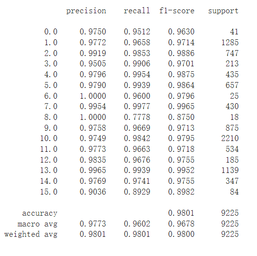
# Generate classification Report
classification = classification_report(ytest, y_pred_test, digits=4)
print(classification)

Alternate function ¶
The following is the standby function used to calculate the accuracy of each class and display the results for reference

from operator import truediv

def AA_andEachClassAccuracy(confusion_matrix):
    counter = confusion_matrix.shape[0]
    list_diag = np.diag(confusion_matrix)
    list_raw_sum = np.sum(confusion_matrix, axis=1)
    each_acc = np.nan_to_num(truediv(list_diag, list_raw_sum))
    average_acc = np.mean(each_acc)
    return each_acc, average_acc


def reports (test_loader, y_test, name):
    count = 0
    # Model test
    for inputs, _ in test_loader:
        inputs = inputs.to(device)
        outputs = net(inputs)
        outputs = np.argmax(outputs.detach().cpu().numpy(), axis=1)
        if count == 0:
            y_pred =  outputs
            count = 1
        else:
            y_pred = np.concatenate( (y_pred, outputs) )

    if name == 'IP':
        target_names = ['Alfalfa', 'Corn-notill', 'Corn-mintill', 'Corn'
                        ,'Grass-pasture', 'Grass-trees', 'Grass-pasture-mowed', 
                        'Hay-windrowed', 'Oats', 'Soybean-notill', 'Soybean-mintill',
                        'Soybean-clean', 'Wheat', 'Woods', 'Buildings-Grass-Trees-Drives',
                        'Stone-Steel-Towers']
    elif name == 'SA':
        target_names = ['Brocoli_green_weeds_1','Brocoli_green_weeds_2','Fallow','Fallow_rough_plow','Fallow_smooth',
                        'Stubble','Celery','Grapes_untrained','Soil_vinyard_develop','Corn_senesced_green_weeds',
                        'Lettuce_romaine_4wk','Lettuce_romaine_5wk','Lettuce_romaine_6wk','Lettuce_romaine_7wk',
                        'Vinyard_untrained','Vinyard_vertical_trellis']
    elif name == 'PU':
        target_names = ['Asphalt','Meadows','Gravel','Trees', 'Painted metal sheets','Bare Soil','Bitumen',
                        'Self-Blocking Bricks','Shadows']
    
    classification = classification_report(y_test, y_pred, target_names=target_names)
    oa = accuracy_score(y_test, y_pred)
    confusion = confusion_matrix(y_test, y_pred)
    each_acc, aa = AA_andEachClassAccuracy(confusion)
    kappa = cohen_kappa_score(y_test, y_pred)
    
    return classification, confusion, oa*100, each_acc*100, aa*100, kappa*100

The test results are written in the document:

classification, confusion, oa, each_acc, aa, kappa = reports(test_loader, ytest, 'IP')
classification = str(classification)
confusion = str(confusion)
file_name = "classification_report.txt"

with open(file_name, 'w') as x_file:
    x_file.write('\n')
    x_file.write('{} Kappa accuracy (%)'.format(kappa))
    x_file.write('\n')
    x_file.write('{} Overall accuracy (%)'.format(oa))
    x_file.write('\n')
    x_file.write('{} Average accuracy (%)'.format(aa))
    x_file.write('\n')
    x_file.write('\n')
    x_file.write('{}'.format(classification))
    x_file.write('\n')
    x_file.write('{}'.format(confusion))

The following code is used to display the classification results:

# load the original image
X = sio.loadmat('Indian_pines_corrected.mat')['indian_pines_corrected']
y = sio.loadmat('Indian_pines_gt.mat')['indian_pines_gt']

height = y.shape[0]
width = y.shape[1]

X = applyPCA(X, numComponents= pca_components)
X = padWithZeros(X, patch_size//2)

# Pixel by pixel prediction category
outputs = np.zeros((height,width))
for i in range(height):
    for j in range(width):
        if int(y[i,j]) == 0:
            continue
        else :
            image_patch = X[i:i+patch_size, j:j+patch_size, :]
            image_patch = image_patch.reshape(1,image_patch.shape[0],image_patch.shape[1], image_patch.shape[2], 1)
            X_test_image = torch.FloatTensor(image_patch.transpose(0, 4, 3, 1, 2)).to(device)                                   
            prediction = net(X_test_image)
            prediction = np.argmax(prediction.detach().cpu().numpy(), axis=1)
            outputs[i][j] = prediction+1
    if i % 20 == 0:
        print('... ... row ', i, ' handling ... ...')

Existing doubts