This experiment is based on the CNN network built by ourselves to classify eye state. Originally, it was intended to migrate learning to classify using VGG16 network. However, the effect of the experiment is very poor and the speed is very slow. It should be the blogger's own problem. However, the model of CNN network built by ourselves is very accurate and fast. This article focuses on confusion matrix drawing, something you haven't touched before.

1. Import Library

import tensorflow as tf
import numpy as np
import matplotlib.pyplot as plt
import os,pathlib,PIL
from tensorflow import keras
from tensorflow.keras import layers,models,Sequential

2. Data Loading

The file path where the data is located

data_dir = "E:/tmp/.keras/datasets/Eye_photos"
data_dir = pathlib.Path(data_dir)
img_count = len(list(data_dir.glob('*/*.jpg')))#Total number of pictures

Setup of Hyperparameters

height = 224
width = 224
epochs = 10
batch_size = 64

Build an ImageDataGenerator. In previous experiments, I used to do data enhancement at this step, including left-right flipping, picture flipping at an angle, horizontal flipping, and so on. However, this is not done in this experiment. Because the eye states identified in this study include left, right, front and closed eyes, if data enhancement is made, the left view changes to the right view, so the data does not achieve the enhancement effect, but introduces noise data, which is not worth it.

train_data_gen = tf.keras.preprocessing.image.ImageDataGenerator(
    rescale=1./255,
    validation_split=0.2)#Divide into training and test sets at a ratio of 8:2

Divided into training and test sets

train_ds = train_data_gen.flow_from_directory(
    directory=data_dir,
    target_size=(height,width),
    batch_size=batch_size,
    shuffle=True,
    class_mode='categorical',
    subset='training'
)
test_ds = train_data_gen.flow_from_directory(
    directory=data_dir,
    target_size=(height,width),
    batch_size=batch_size,
    shuffle=True,
    class_mode='categorical',
    subset='validation'
)

Found 3448 images belonging to 4 classes.
Found 859 images belonging to 4 classes.

View labels

all_images_paths = list(data_dir.glob('*'))##"*" matches 0 or more characters
all_images_paths = [str(path) for path in all_images_paths]
all_label_names = [path.split("\\")[5].split(".")[0] for path in all_images_paths]

['close_look', 'forward_look', 'left_look', 'right_look']

3.CNN Network Setup

model = tf.keras.Sequential([
    tf.keras.layers.Conv2D(16,3,padding="same",activation="relu",input_shape=(height,width,3)),
    tf.keras.layers.MaxPooling2D(),
    tf.keras.layers.Conv2D(32,3,padding="same",activation="relu"),
    tf.keras.layers.MaxPooling2D(),
    tf.keras.layers.Conv2D(64,3,padding="same",activation="relu"),
    tf.keras.layers.MaxPooling2D(),
    tf.keras.layers.Flatten(),
    tf.keras.layers.Dense(1024,activation="relu"),
    tf.keras.layers.Dense(512,activation="relu"),
    tf.keras.layers.Dense(4,activation="softmax")
])

Optimizer settings, specific principles can refer to the license plate to identify that blog.

initial_learning_rate = 1e-4
lr_sch = tf.keras.optimizers.schedules.ExponentialDecay(
    initial_learning_rate=initial_learning_rate,
    decay_rate=0.96,
    decay_steps=20,
    staircase=True
)

The way loss values are calculated is described in the last blog post.

model.compile(
    optimizer=tf.keras.optimizers.Adam(learning_rate=lr_sch),
    loss=tf.keras.losses.CategoricalCrossentropy(),
    metrics=['accuracy']
)

history = model.fit(
    train_ds,
    validation_data=test_ds,
    epochs=epochs
)

The results are as follows:

With epochs=20, the accuracy of the model is about 93%, which is considerable.

Save the model:

model.save("E:/tmp/.keras/datasets/model.h5")

Load Model

new_model = tf.keras.models.load_model("E:/tmp/.keras/datasets/model.h5")

Use models to predict pictures:

plt.figure(figsize=(10,5))
plt.suptitle("Forecast Results Display")
for images,labels in test_ds:
    for i in range(8):
        ax = plt.subplot(2,4,i+1)
        plt.imshow(images[i])
        img_array = tf.expand_dims(images[i],0)#Add one dimension
        pre = new_model.predict(img_array)
        plt.title(all_label_names[np.argmax(pre)])
        plt.axis("off")
    break
plt.show()

4. Confusion Matrix

Confusion matrix, also known as error matrix, is a standard format for accuracy evaluation and is expressed as a matrix of n rows and n columns. In image accuracy evaluation, it is mainly used to compare the classification results with the actual measured values. The accuracy of the classification results can be displayed in a confusion matrix. The confusion matrix is calculated by comparing the location and classification of each measured cell with the corresponding location and classification in the classified image.
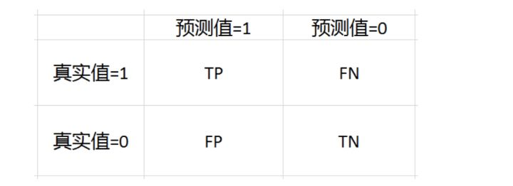
The most familiar confusion matrix is the two-class confusion matrix:

TP = True Postive = True Positive; FP = False Positive = False Positive

FN = False Negative = false negative; TN = True Negative = True Negative

As for the multiclass confusion matrix, it is similar to the two-class confusion matrix. Let's draw a confusion matrix for eye state recognition.

sns.heatmap is the main tool used to draw the confusion matrix, which is a method under the seaborn package, as follows:

seaborn.heatmap(data, vmin=None, vmax=None, cmap=None, center=None, robust=False, annot=None, fmt='.2g', annot_kws=None, linewidths=0, linecolor='white', cbar=True, cbar_kws=None, cbar_ax=None, square=False, xticklabels='auto', yticklabels='auto', mask=None, ax=None, **kwargs)

In fact, all parameters except the first parameter, data, are default parameters and can be ignored. Here, if you receive a clean two-dimensional numpy array, you can see that the row label is 0,1,2, and if it is a DataFrame, you can mark it with the column name.

Libraries needed

from sklearn.metrics import confusion_matrix
import seaborn as sns
import pandas as pd

Define a function to draw the confusion matrix

#Draw confusion matrix
def plot_cm(labels,pre):
    conf_numpy = confusion_matrix(labels,pre)#Draw confusion matrix based on actual and predicted values
    conf_df = pd.DataFrame(conf_numpy,index=all_label_names,columns=all_label_names)#Put data and all_label_names made into DataFrame s
    plt.figure(figsize=(8,7))

    sns.heatmap(conf_df,annot=True,fmt="d",cmap="BuPu")#Draw data as confusion matrix
    plt.title('Confusion Matrix',fontsize = 15)
    plt.ylabel('True Value',fontsize = 14)
    plt.xlabel('predicted value',fontsize = 14)
    plt.show()

Get predicted and actual values

test_pre = []
test_label = []
for images,labels in test_ds:
    for image,label in zip(images,labels):
        img_array = tf.expand_dims(image,0)#Add a common dimension
        pre = new_model.predict(img_array)#Forecast results
        test_pre.append(all_label_names[np.argmax(pre)])#Pass predictions into the list
        test_label.append(all_label_names[np.argmax(label)])#Pass real results into the list
    break#Due to hardware problems. I only use one batch here, 64 pictures in total.
plot_cm(test_label,test_pre)#Draw confusion matrix

Try to refuel a