I. Research on Related Algorithms

1.1 Common Open Source Algorithms
- Yahoo: EGADS
- FaceBook: Prophet
- Baidu: Opprentice
- Twitter: Anomaly Detection
- Redhat: hawkular
- Ali+Tsinghua: Donut
- Tencent: Metis
- Numenta: HTM
- CMU: SPIRIT
- Microsoft: YADING
- Linkedin: Improved version of SAX
- Netflix: Argos
- NEC: CloudSeer
- NEC+Ant: LogLens
- MoogSoft: A start-up company. The content is very good for your reference.
1.2 Anomaly Detection Based on Statistical Method
Based on the statistical method, the results of different indicators (mean, variance, divergence, kurtosis, etc.) of the time series data are discriminated, and the warning is carried out by setting threshold through certain artificial experience. At the same time, time series historical data can be introduced to alarm by using ring ratio and year-on-year strategy and setting threshold through certain artificial experience.
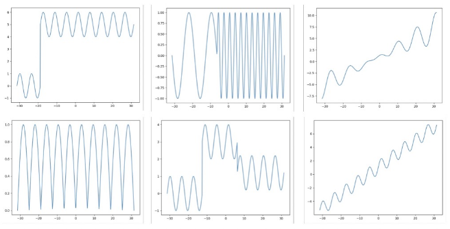
By establishing different statistical indicators: window mean change, window variance change and so on, we can better solve the abnormal point detection corresponding to (1, 2, 5) in the following figure; we can detect the corresponding cusp information of (4) by local extremum; we can better find the corresponding change trend of (3, 6) in the graph by time series prediction model. Potential, detect abnormal points that do not conform to the law.
How to distinguish anomalies?
- N-sigma
- Boxplot
- Grubbs'Test
- Extreme Studentized Deviate Test
PS:
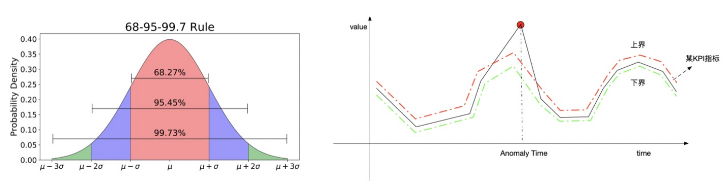
- N-sigma: In normal distribution, 99.73% of the data are within three standard deviations from the average. If our data obey a certain distribution, we can infer the probability of the current value from the distribution curve.
- Grubbs hypothesis test: often used to test single outliers in normal distribution data sets
- ESD Hypothesis Testing: Grubbs'
- Test extends to k outlier detection
1.3 Anomaly Detection Based on Unsupervised Method
What is an unsupervised method: whether there is supervision or not, mainly depends on whether the data modeled is label or not. If the input data is labeled, supervised learning occurs; unsupervised learning occurs without labels.
Why do we need to introduce unsupervised methods: In the early stage of monitoring establishment, user feedback is very rare and precious. Without user feedback, in order to quickly establish reliable monitoring strategies, unsupervised methods are introduced.
For Single Dimension Indicators
- Some regression methods (Holt-Winters, ARMA) are used to learn the prediction sequence from the original observation sequence, and the related anomalies are obtained by analyzing the residual between them.
-
For Single Dimension Indicators
- Multidimensional Meaning (time, cpu, iops, flow)
-
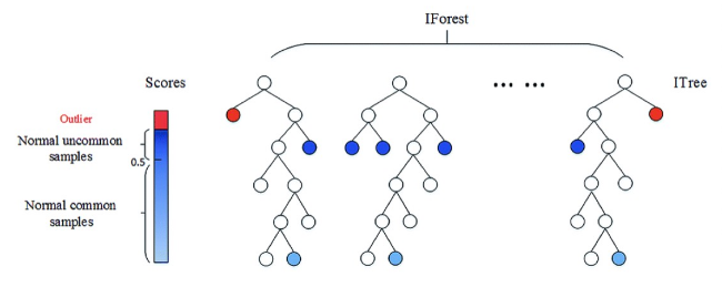
iForest (Isolation Forest) is an integrated anomaly detection method
- Suitable for continuous data, with linear time complexity and high accuracy
- Definition of anomalies: outliers that are easily isolated, points that are sparsely distributed and far from densely populated groups.
-
Several explanations
- The more discriminant trees, the more stable they are, and each tree is independent of each other. It can be deployed in a large-scale distributed system.
- The algorithm is not suitable for particularly high-dimensional data, and noise dimension and sensitive dimension can not be removed actively.
- The original iForest algorithm is only sensitive to global outliers, but less sensitive to locally sparse points.
1.4 Anomaly Detection Based on Deep Learning
Title: Unsupervised Anomaly Detection via Variational Auto-Encoder for Seasonal KPIs in Web Applications (WWW 2018)
- Solution: For periodic time series monitoring data, the data contains some missing points and outliers.
- The model training structure is as follows

- MCMC filling technology is used to deal with the known missing points in the observation window. The core idea is to iteratively approximate the marginal distribution based on the trained model (the following chart shows an iteration diagram filled by MCMC).

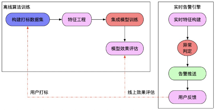
1.5 Use supervised methods for anomaly detection
-
Is the annotation of anomalies complex in itself?
- User-defined anomalies are often marked from the system or service point of view. The underlying indicators and link indicators associated are complex and can not be started from several dimensions (more is a Shapshot of the system).
- When designing the architecture layer, service self-healing design will be carried out, and the underlying anomalies will not affect the upper business.
- The traceability of anomalies is complex. In many cases, a single monitoring data is only a response to the anomaly results, not the anomaly itself.
- The number of labeled samples is very small, and the types of anomalies are various. The learning problems for small samples need to be improved.
-
Commonly used supervised machine learning methods
- xgboost, gbdt, lightgbm, etc.
- Some classified networks of dnn, etc.
2. Algorithmic Ability Provided in SLS
-
Time series analysis
- Prediction: Fitting baselines based on historical data
- Anomaly Detection, Change Point Detection, Break Point Detection: Finding Anomaly Points
- Multi-cycle Detection: Discovering Periodic Rules in Data Access
- Time Series Clustering: Finding Time Series with Different Forms
-
pattern analysis
- Frequent pattern mining
- Differential pattern mining

-
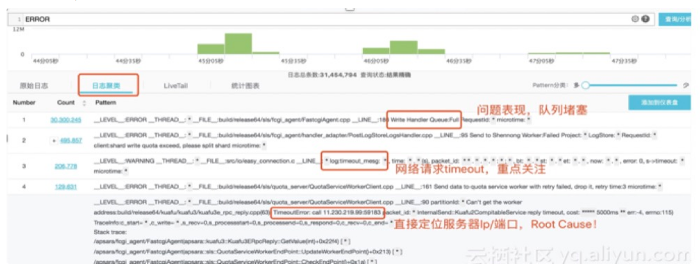
Intelligent Clustering of Massive Texts
- Support arbitrary format logs: Log4J, Json, single line (syslog)
- Logs are filtered under arbitrary conditions and then reduced; For Reduce post-Pattern, the original data is checked according to signature.
- Pattern s comparison in different time periods
- Dynamic Adjustment of Reduce Accuracy
- Billion-level data, second-level results
3. Actual combat analysis for traffic scenarios
3.1 Visualization of Multidimensional Monitoring Indicators
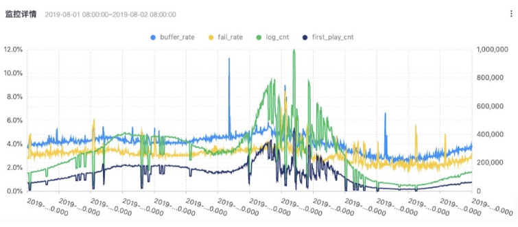
Specific SQL logic is as follows:
* |
select
   time,
   buffer_cnt,
   log_cnt,
   buffer_rate,
   failed_cnt,
   first_play_cnt,
   fail_rate
from
   (
      select
         date_trunc('minute', time) as time,
         sum(buffer_cnt) as buffer_cnt,
         sum(log_cnt) as log_cnt,
         case
            when
               is_nan(sum(buffer_cnt)*1.0 / sum(log_cnt))
            then
               0.0
            else
               sum(buffer_cnt)*1.0 / sum(log_cnt)
         end as buffer_rate,
sum(failed_cnt) as failed_cnt,
sum(first_play_cnt) as first_play_cnt ,
         case
            when
               is_nan(sum(failed_cnt)*1.0 / sum(first_play_cnt))
            then
               0.0
            else
               sum(failed_cnt)*1.0 / sum(first_play_cnt)
         end as fail_rate
      from
         log
      group by
         time
      order by
         time
   )
   limit 100000
3.2 Time Series Ring Ratio Diagram of Indicators

Specific SQL logic is as follows:
* |
select
    time,
    log_cnt_cmp[1] as log_cnt_now,
    log_cnt_cmp[2] as log_cnt_old,
    case when is_nan(buffer_rate_cmp[1]) then 0.0 else buffer_rate_cmp[1] end as buf_rate_now,
    case when is_nan(buffer_rate_cmp[2]) then 0.0 else buffer_rate_cmp[2] end as buf_rate_old,
    case when is_nan(fail_rate_cmp[1]) then 0.0 else fail_rate_cmp[1] end as fail_rate_now,
    case when is_nan(fail_rate_cmp[2]) then 0.0 else fail_rate_cmp[2] end as fail_rate_old
from
(
select
    time,
    ts_compare(log_cnt, 86400) as log_cnt_cmp,
    ts_compare(buffer_rate, 86400) as buffer_rate_cmp,
    ts_compare(fail_rate, 86400) as fail_rate_cmp
from (
select
      date_trunc('minute', time - time % 120) as time,
    sum(buffer_cnt) as buffer_cnt,
    sum(log_cnt) as log_cnt,
    sum(buffer_cnt)*1.0 / sum(log_cnt) as buffer_rate,
    sum(failed_cnt) as failed_cnt,
    sum(first_play_cnt) as first_play_cnt ,
    sum(failed_cnt)*1.0 / sum(first_play_cnt) as fail_rate
from log group by time order by time) group by time)
where time is not null limit 1000000
3.3 Dynamic Visualization of Indicators

Specific SQL logic is as follows:
* |
select
    time,
    case when is_nan(buffer_rate) then 0.0 else buffer_rate end as show_index,
    isp as index
from
(select
    date_trunc('minute', time) as time,
    sum(buffer_cnt)*1.0 / sum(log_cnt) as buffer_rate,
    sum(failed_cnt)*1.0 / sum(first_play_cnt) as fail_rate,
    sum(log_cnt) as log_cnt,
    sum(failed_cnt) as failed_cnt,
    sum(first_play_cnt) as first_play_cnt,
    isp
from log group by time, isp order by time) limit 200000
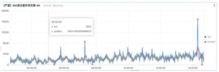
3.4 Monitoring Dashboard page for exception sets

- Diagram SQL logic behind exception monitoring projects
* |
select
    res.name
from (
    select
        ts_anomaly_filter(province, res[1], res[2], res[3], res[6], 100, 0) as res
    from (
        select
            t1.province as province,
            array_transpose( ts_predicate_arma(t1.time, t1.show_index, 5, 1, 1) ) as res
        from (
            select
                province,
                time,
                case when is_nan(buffer_rate) then 0.0 else buffer_rate end as show_index
            from (
                select
                    province,
                    time,
                    sum(buffer_cnt)*1.0 / sum(log_cnt) as buffer_rate,
                    sum(failed_cnt)*1.0 / sum(first_play_cnt) as fail_rate,
                    sum(log_cnt) as log_cnt,
                    sum(failed_cnt) as failed_cnt,
                    sum(first_play_cnt) as first_play_cnt
                from log
                group by province, time) ) t1
            inner join (
                select
                    DISTINCT province
                from  (
                    select
                        province, time, sum(log_cnt) as total
                    from log
                    group by province, time )
                where total > 200 ) t2 on t1.province = t2.province
        group by t1.province ) ) limit 100000
- Specific analysis of the above-mentioned SQL logic

Links to the original text
This article is the original content of Yunqi Community, which can not be reproduced without permission.