1 exploratory data analysis
Data were used: Pima Indian diabetes prediction dataset.
Link: https://pan.baidu.com/s/17M7UfnqGYTkpLmCXUOyTkw
Extraction code: y4fz
import pandas as pd
pima_column_names = ['times_pregnant', 'plasma_glucose_concentration',
                     'diastolic_blood_pressure', 'triceps_thickness',
                     'serum_insulin', 'bmi', 'pedigree_function',
                     'age', 'onset_diabetes']
pima = pd.read_csv('./data/pima.data', names=pima_column_names)
- times_pregnant: number of pregnancies;
- plasma_glucose_concentration: 2-hour plasma glucose concentration in oral glucose tolerance test;
- diastolic_blood_pressure: diastolic blood pressure (mmHg);
- triceps_thickness: triceps skinfold thickness (mm);
- serum_insulin: 2-hour serum insulin concentration( μ U/ml);
- BMI: body mass index (BMI, c);
- pedigree_function: family function of diabetes;
- Age: age (years);
- onset_diabetes: tag (0 or 1, no or diabetes).
pima['onset_diabetes'].value_counts(normalize=True)
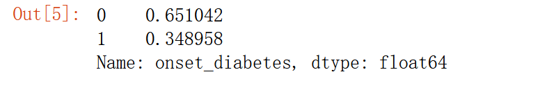
65% had no diabetes.
Null accuracy refers to the accuracy achieved when the model always predicts categories with high frequency
The empty accuracy rate is to directly predict all data into the largest number of classes without training models (0 in this column: no diabetes).
If the accuracy of the trained model is less than 65%, that is, the empty accuracy, then it can be said that our model is almost worthless.
2 explore the blood glucose concentration of different types of samples
We can view the comparison of various characteristics of samples in different categories
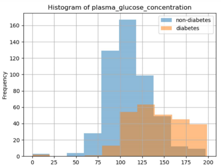
2-hour plasma glucose concentration in oral glucose tolerance test
import matplotlib.pyplot as plt
col = 'plasma_glucose_concentration'
plt.hist(pima[pima['onset_diabetes'] == 0][col], 10, alpha=0.5, label='non-diabetes')
plt.hist(pima[pima['onset_diabetes'] == 1][col], 10, alpha=0.5, label='diabetes')
plt.legend(loc='upper right')
plt.xlabel(col)
plt.ylabel('Frequency')
plt.title('Histogram of {}'.format(col))
plt.grid()
Histogram distribution of several anomalies (except 1)
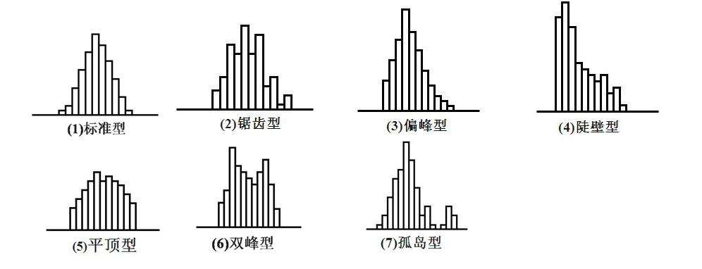 It can be seen that the drawn graph belongs to the 7 islanding data anomaly, and it can also be seen that the blood glucose level of normal people is 75-125, while that of diabetic patients is 100-175.. It indicates that blood glucose concentration can be used to identify diabetes mellitus to some extent.
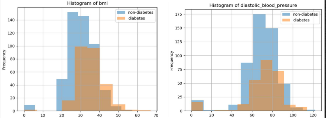
Similarly, body mass index (bmi) and diastolic_blood_pressure can be plotted
3. Missing value exploration
Problems caused by missing values
1 most machine learning algorithms cannot handle missing values
2 missing information
pima.isnull().sum()
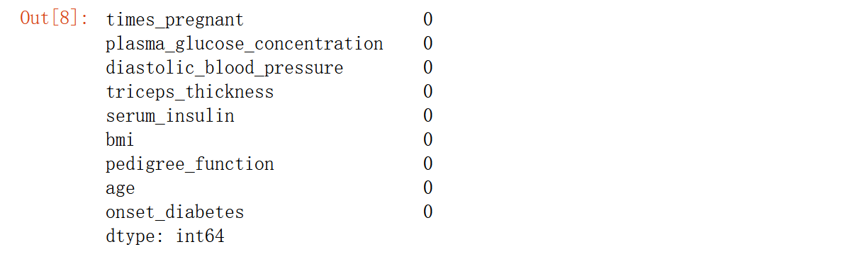 It seems that there is no missing value, but it is also possible that the missing value has been filled with 0, so let's explore further
# Is there really no missing value
pima.describe()
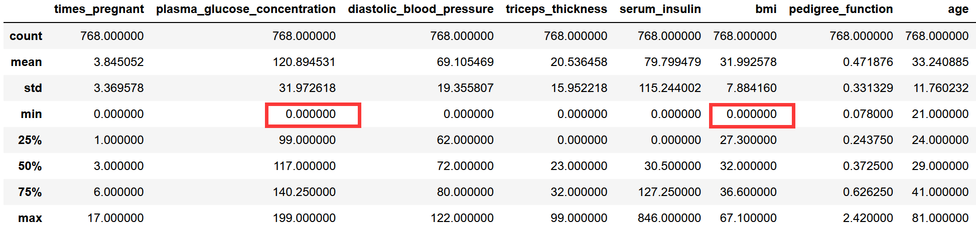
According to common sense, bmi and blood glucose concentration cannot be 0
The following minimum values are 0:
- times_pregnant: number of pregnancies;
- plasma_glucose_concentration: 2-hour plasma glucose concentration in oral glucose tolerance test;
- diastolic_blood_pressure: diastolic blood pressure (mmHg);
- triceps_thickness: triceps skinfold thickness (mm);
- serum_insulin: 2-hour serum insulin concentration( μ U/ml);
- BMI: body mass index (BMI, i.e. weight (kg) divided by the square of height (m));
- onset_diabetes: tag (0 or 1, no or diabetes).
Maybe the missing or nonexistent values in the original dataset are filled with 0!
The tag column and the number of pregnancies may be 0, while other columns cannot have a value of 0. Therefore, the following fields originally have missing values!
- plasma_glucose_concentration: 2-hour plasma glucose concentration in oral glucose tolerance test;
- diastolic_blood_pressure: diastolic blood pressure (mmHg);
- triceps_thickness: triceps skinfold thickness (mm);
- serum_insulin: 2-hour serum insulin concentration( μ U/ml);
- BMI: body mass index (BMI, i.e. weight (kg) divided by the square of height (m)).
Therefore, replace the 0 in the above column with the missing value
# Use None to replace the 0 in the above column to achieve the effect of the original state of the data
columns = ['serum_insulin', 'bmi', 'plasma_glucose_concentration', 'diastolic_blood_pressure', 'triceps_thickness']
for colu in columns:
    pima[colu].replace([0], [None], inplace=True)
pima.isnull().sum()

4. Delete missing values
Processing missing values
1. Delete missing values
2 fill in missing values
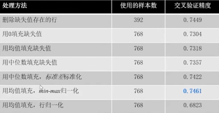
You can see the performance of the model under different treatments ()
The first is to delete missing values
pima_dropped = pima.dropna()
pima_dropped.shape
 The original data is (768, 9), and many samples are lost by direct deletion
Then look at the change of sample data distribution before and after deletion
(pima_dropped.mean() - pima.mean())/pima.mean()
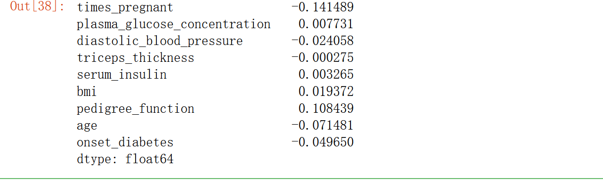
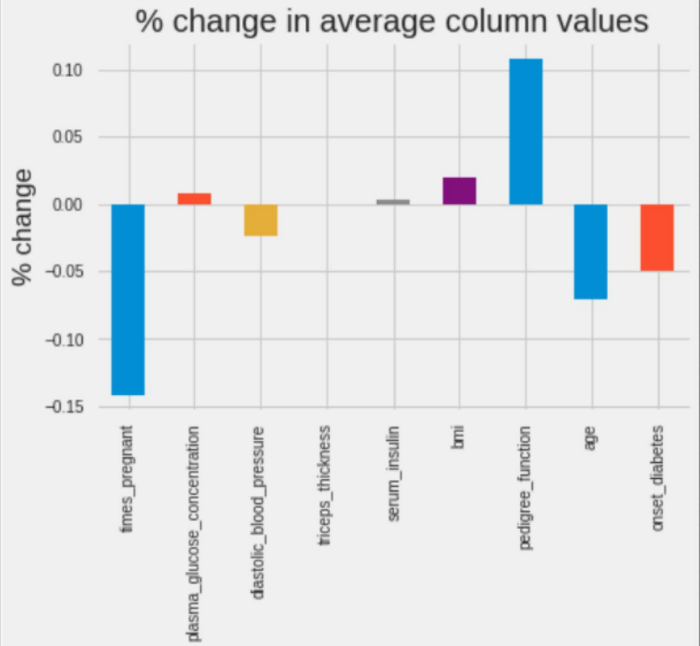 times_ The mean pregnant (number of pregnancies) decreased by 14% pedigree_function (diabetic blood function) increased by 11%.
Deleting samples can seriously affect the shape of the data, so you should keep as much data as possible.
How we know the effect of direct deletion can be evaluated by the performance of the model
5 build baseline model
from sklearn.neighbors import KNeighborsClassifier
from sklearn.model_selection import cross_val_score
X_dropped = pima_dropped.drop('onset_diabetes', axis=1)
y_dropped = pima_dropped['onset_diabetes']
knn=KNeighborsClassifier(n_neighbors=3)
cross_val_score(knn,X_dropped,y_dropped,cv=5).mean()

6. Grid optimization
When setting parameters, we do not know how many parameters are most appropriate, such as n just now_ It's easy to think of loops
for k in range(1, 8):
    for cv in range(2,5):
        knn = KNeighborsClassifier(n_neighbors=k)
        accuracy = cross_val_score(knn, X_dropped, y_dropped, cv=5).mean()
        print(accuracy)
But when there are more than three parameters? In fact, there is a grid search interface in sklearn that can be called. Grid search (enumerate each combination as the name suggests, just like grid)
Grid search can be used in this relatively simple model, but modeling competition, XGboost and lightGBM do not recommend grid search. You can try random search and Bayesian search. The following is the grid search interface call in sklearn
from sklearn.model_selection import GridSearchCV
knn_params = {'n_neighbors': [1, 2, 3, 4, 5, 6, 7]}
grid = GridSearchCV(KNeighborsClassifier(), knn_params)
grid.fit(X_dropped, y_dropped)
grid.best_estimator_   # model parameter
grid.best_score_    # Model performance baseline

7. Fill in the missing values with 0 / mean
Filling in missing values with 0 is actually the first public data set obtained
pima_fill_zero = pima.fillna(0)
X_fill_zero = pima_fill_zero.drop('onset_diabetes', axis=1)
y_fill_zero = pima_fill_zero['onset_diabetes']
grid_zero = GridSearchCV(KNeighborsClassifier(), knn_params)
grid_zero.fit(X_fill_zero, y_fill_zero)
grid_zero.best_score_
 In addition to filling with 0, you can also fill with mean or interpolation
from sklearn.impute import SimpleImputer
pima_fill_mean = SimpleImputer(strategy='mean').fit_transform(pima)
X_fill_mean = pima_fill_mean[:, :-1]
y_fill_mean = pima_fill_mean[:, -1]
grid_mean = GridSearchCV(KNeighborsClassifier(), knn_params)
grid_mean.fit(X_fill_mean, y_fill_mean)
grid_mean.best_score_
 In addition to filling in the missing data values, you can also annotate the data to improve the model
8. Introduction to standardization and normalization
data standardization means that in the multi index evaluation system, due to the different nature of each evaluation index, it usually has different dimensions and orders of magnitude. When the level of each index varies greatly, if the original index value is directly used for analysis, it will highlight the role of the index with higher value in the comprehensive analysis and relatively weaken the role of the index with lower value level. Therefore, in order to ensure the reliability of the results, it is necessary to standardize the original index data
Role of standardization
Improve model performance; Accelerate learning efficiency
Common standardization methods
1. Z-score standardization / feature standardization / variance scaling; Standardization of standard deviation
2 min max normalization / min max scaling (mapping between [0,1] intervals)
3 rows normalized.
The first two are column alignment and the last one is row alignment
1. Standardization of Z scores
By scaling features, unifying the mean and variance (square of standard deviation) Ø Z scores, the standardized output will be rescaled to make the mean 0 and standard deviation 1. Standardization and normalization of Z-scores
z=(x-u)/σ
The 2min Max normalization is similar to the Z-score normalization because it also replaces each value in the column with a formula.
The use of these two methods is introduced
3. Row normalization
This standardized method is about rows. Row normalization does not calculate the statistical values (mean, minimum, maximum, etc.) of each column, but ensures that each row has a unit norm, which means that the vector length of each row is the same.
x
=
(
x
1
,
x
2
,
x
3
.
.
.
.
.
x
n
)
x=(x_1,x_2,x_3.....x_n)
x=(x1,x2,x3.....xn)
||x||
=
(
x
1
2
+
x
2
2
+
.
.
.
.
.
x
n
2
)
2
=\sqrt[2]{(x_1^2+x_2^2+.....x_n^2)}
=2(x12+x22+.....xn2)
X_new=x/||x||
from sklearn.preprocessing import Normalizer # Row normalization
normalize = Normalizer()
pima_normalized = pd.DataFrame(normalize.fit_transform(pima_imputed), columns=pima_column_names)
np.sqrt((pima_normalized**2).sum(axis=1)).mean()# Average norm of matrix after row normalization
Of course, not all models are affected by dimensions
Algorithm affected by scale
1KNN: because it depends on Euclidean distance;
2. Mean clustering: the same reason as KNN;
3 logistic regression, support vector machine, neural network: if gradient descent is used to learn weight;
4 principal component analysis: the feature vector will be biased towards larger columns.
9. Further optimization combined with machine learning pipeline
As the follow-up work progresses, the model needs to do more and more processing. We can put these processes into the pipeline.
from sklearn.pipeline import Pipeline
from sklearn.preprocessing import StandardScaler, MinMaxScaler
X = pima.drop('onset_diabetes', axis=1)
y = pima['onset_diabetes']
pipeline = Pipeline(steps=[('imputer', SimpleImputer()), ('standardize', MinMaxScaler()), ('classify', KNeighborsClassifier())])  # SimpleImputer is used for filling, MinMaxScaler is used for standardization, and KNN is used for model classification
pipeline_params = {'imputer__strategy': ['mean', 'median'], 'classify__n_neighbors': [1, 2, 3, 4, 5, 6, 7]}   # Parameter table
grid_pipeline = GridSearchCV(pipeline, pipeline_params)
grid_pipeline.fit(X, y)
grid_pipeline.best_estimator_, grid_pipeline.best_score_
 Note that the objects placed in the Pipeline must have fit,fit_transform method
Note the parameter format and step name in the parameter table__ Parameters, such as the strategy parameter in imputer, set imputer__strategy
10 summary
Identify missing values
Process missing values (delete, 0 fill, statistics fill)
Data standardization
Machine learning pipeline
The specific method to deal with missing values needs to be tried