be careful:

1. All the articles in this series are mainly developed by the gradient lifting tree model. The extracted features are mainly to help the gradient lifting tree model mine the information it can't mine. All the features introduced in this paper can be directly added to the model as features, which is slightly different from the strategy based on neural network;

2. Due to too much space, this article introduces 20 different features of text features, and the subsequent text features will be updated in the following articles!

 

Text features - Part I

There will be some simple intersection between text features and category features. Some simple text features can be directly treated as category features, for example:

• Flower color: red, blue, yellow, etc;

• Names: Mr jack, Mr smith, Mr will, Mr phil, etc.

These features can be directly Label coded, and then feature engineering can be carried out by using the skill of category features. In addition to treating text features as category features, we need to pay attention to a lot of details when doing text related feature engineering. Compared with Label coding, it is how to prevent the loss of information in the text. The processing of text features involves a lot of NLP technologies. Here we mainly introduce some places that often need attention and some skills. For the latest methods, you can follow up the latest NLP related technologies.

For the feature engineering of text features based on the gradient lifting tree model, we need to fully mine the information lost in Label coding, such as the name feature above, there are very strong internal laws, Mr and other information. These information reflect gender related information. If Label coding is carried out directly, such information will be lost, So we can mine it through text skills.

1.expansion code

expansion code often appears in some complex strings, such as some strings with version information. Many version number information includes time, number and other information. We need to separate them to form multiple new feature columns, such as the following example:

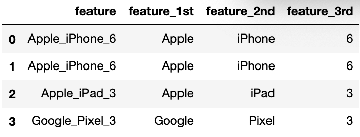
expansion coding is similar to clustering information with business information. It can accelerate the search speed of tree model, and it is also a very good feature

import pandas as pd
df = pd.DataFrame()
df['feature']      = ['Apple_iPhone_6', 'Apple_iPhone_6', 'Apple_iPad_3', 'Google_Pixel_3']
df['feature_1st']  = df['feature'].apply(lambda x: x.split('_')[0])
df['feature_2nd']  = df['feature'].apply(lambda x: x.split('_')[1])
df['feature_3rd']  = df['feature'].apply(lambda x: x.split('_')[2])
df

	feature	feature_1st	feature_2nd	feature_3rd
0	Apple_iPhone_6	Apple	iPhone	6
1	Apple_iPhone_6	Apple	iPhone	6
2	Apple_iPad_3	Apple	iPad	3
3	Google_Pixel_3	Google	Pixel	3

2.consolidation code

consolidation code often appears in some special strings, such as:

• Some strings with addresses will give detailed information, such as No. XX, XX village, XX County, XX city. At this time, we can extract the city as a new feature;

• Many products, such as mobile phones, pad s, etc., can be abstracted as information of apple, Samsung and other companies;

 

consolidation code is similar to the above expansion code. It is also a kind of clustering information with business information, which can accelerate the search speed of tree model. It is also a very good feature

3. Text length features

The length features of the text can be enumerated according to the four granularity of paragraphs, sentences, words and letters of the text. These features can reflect the paragraph structure of the text and are very important information in many problems, such as judging the type of text, whether the text is a novel or a paper or others. At this time, the length feature of the text is a very strong feature.

 

1. Number of paragraphs

As the name suggests, it is the number of paragraphs in the text.

2. Number of sentences

The number of sentences in the text can be counted by calculating the number of periods and exclamation marks.

3. Number of words

The number of words in the text can be calculated by directly converting punctuation marks into spaces and then calculating the number of spaces.

4. Number of letters

After deleting all punctuation, count the number of all letters directly.

5. Average number of sentences in each paragraph

Average number of sentences per paragraph = number of sentences / number of paragraphs

6. Average number of words in each paragraph

Average number of sentences per paragraph = number of words / number of paragraphs

7. Average number of letters per paragraph

Average number of sentences per paragraph = number of text letters / number of paragraphs

8. Average number of words in each sentence

Average number of words per sentence = number of words / number of sentences

9. Average number of letters in each sentence

Average number of letters per sentence = number of text letters / number of sentences

10. Average length of each word

Average length of each word = number of text letters / number of text words

4. Punctuation features

Punctuation also contains very important information. For example, in the problem of emotion classification, exclamation marks and other information often mean very strong emotional expression, which can bring great help to the prediction of the final model.

1. Number of punctuation marks

Directly calculate the number of times punctuation occurs.

2. Number of special punctuation marks

Count the occurrence times of some important punctuation marks in the text, for example:

• In the problem of emotion classification, the number of exclamation marks and question marks.

• The number of abnormal symbols in the virus prediction problem.

3. Others

Here, we need to pay extra attention to some strange punctuation marks, such as continuous exclamation marks, "!!!" Or multiple consecutive question marks'??? ', The emotional expression of this symbol is stronger, so it also needs special attention many times.

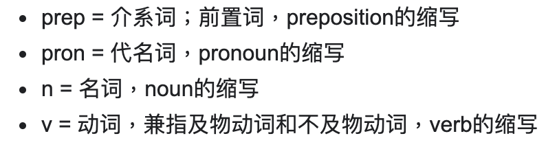
5. Lexical attribute characteristics

Each word has its own attribute, such as noun, verb, adjective and so on. Lexical attribute features can often help the model to bring a slight improvement in effect, and can be used as a kind of supplementary information.

‍

‍

6. Special lexical features

Punctuation can reflect the emotional intensity and other information of the text from the side. It plays a very important role in emotional classification and text classification. Of course, at the same time, the characteristics of special words are more important.

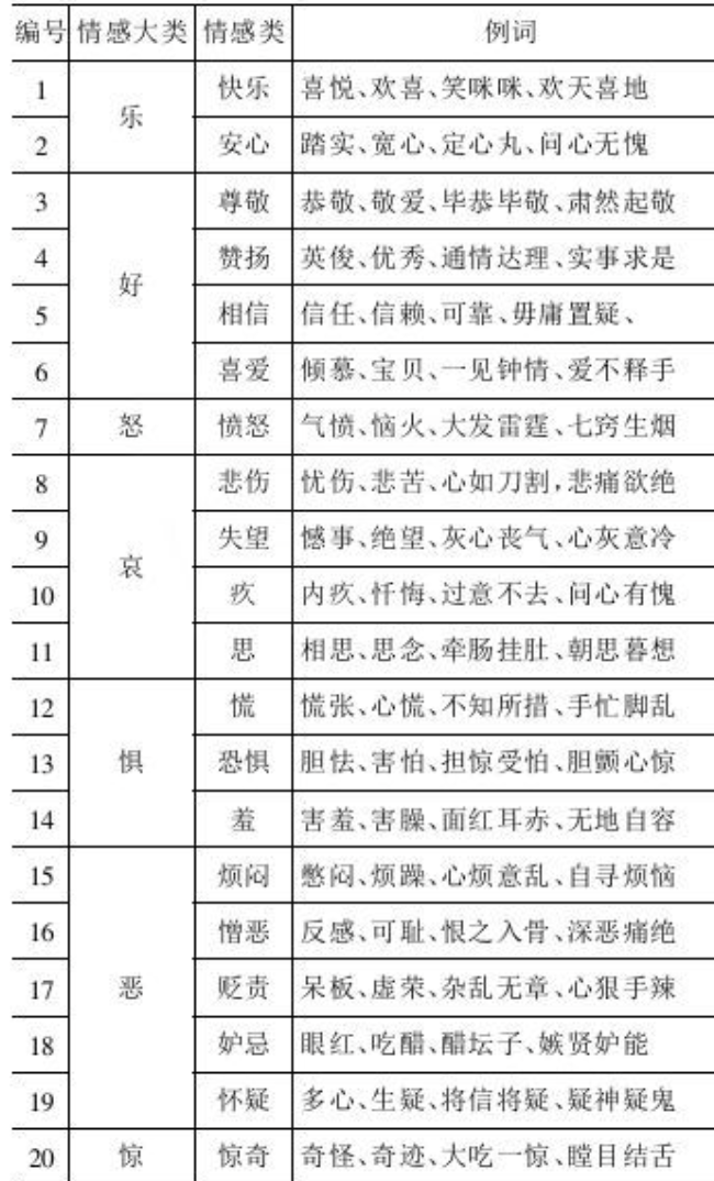
We can choose to count the number of words in each category directly by category (each category represents one category of emotion).

7. Word frequency characteristics

The above are some simple text features, and some text information will be relatively complex, such as sentences and other texts. At this time, we need some common text tools, and the most common is the word frequency statistical feature. This feature is relatively simple, which is to count the number of occurrences of each word in the text, because each text is generally composed of words, and the number of occurrences of each word can reflect the content of the article to a certain extent, for example, in a planning article, The word "love" appears more often, that is to say, the word frequency corresponding to "love" is relatively large, so we can guess that the article is likely to belong to emotional articles. Therefore, when dealing with text information, word frequency feature is one of the very important information.

#Import Toolkit
from sklearn.feature_extraction.text import CountVectorizer 
#Initialize and introduce stop vocabulary
vectorizer = CountVectorizer(stop_words=set(['the', 'six', 'less', 'being', 'indeed', 'over', 'move', 'anyway', 'four', 'not', 'own', 'through', 'yourselves']))
df = pd.DataFrame()
df['text'] = ["The sky is blue.", "The sun is bright.","The sun in the sky is bright.", "We can see the shining sun, the bright sun."]
 
#Get vocabulary
vectorizer.fit_transform(df['text']).todense()

matrix([[1, 0, 0, 0, 1, 0, 0, 1, 0, 0],
        [0, 1, 0, 0, 1, 0, 0, 0, 1, 0],
        [0, 1, 0, 1, 1, 0, 0, 1, 1, 0],
        [0, 1, 1, 0, 0, 1, 1, 0, 2, 1]])

If you want to know the meaning of each column above, you can directly observe the dictionary of the text.

vectorizer.vocabulary_

{'sky': 7,
 'is': 4,
 'blue': 0,
 'sun': 8,
 'bright': 1,
 'in': 3,
 'we': 9,
 'can': 2,
 'see': 5,
 'shining': 6}

Word frequency features are simple and easy to understand, and can capture text information from a macro perspective. Compared with direct Label coding, it can extract more useful information features, thus improving the effect. However, word frequency features are often affected by stop words. For example, "the,a" often appears more times. If the wrong clustering distance is selected, such as l2 distance, it is often difficult to obtain better clustering effect, Therefore, it is necessary to carefully delete and select words; Affected by the size of the text, if the article is long, there will be more words, the text is short, and there will be fewer words.

8.TF-IDF features

TF-IDF feature is an extension of word frequency feature. Word frequency feature can represent text information from a macro perspective, but in word frequency method, the role of frequent words is amplified, such as common "I",'the '; reduces the role of rare words, such as "garden" and "tiger", but these words have a very important amount of information, so word frequency features are often difficult to capture some information that appears less frequently but is very effective. TF-IDF features can be a good way to alleviate such problems. TF-IDF from global (all files) and local (single file) To solve the above problems, TF-IDF can better give the importance of a word to a file.

from sklearn.feature_extraction.text import TfidfVectorizer

tfidf_model = TfidfVectorizer()
#Get vocabulary
tfidf_matrix = tfidf_model.fit_transform(df['text']).todense()
tfidf_matrix

matrix([[0.65919112, 0.        , 0.        , 0.        , 0.42075315,
         0.        , 0.        , 0.51971385, 0.        , 0.34399327,
         0.        ],
        [0.        , 0.52210862, 0.        , 0.        , 0.52210862,
         0.        , 0.        , 0.        , 0.52210862, 0.42685801,
         0.        ],
        [0.        , 0.3218464 , 0.        , 0.50423458, 0.3218464 ,
         0.        , 0.        , 0.39754433, 0.3218464 , 0.52626104,
         0.        ],
        [0.        , 0.23910199, 0.37459947, 0.        , 0.        ,
         0.37459947, 0.37459947, 0.        , 0.47820398, 0.39096309,
         0.37459947]])

If you want to know the meaning of each column above, you can directly observe the dictionary of the text.

tfidf_model.vocabulary_

{'the': 9,
 'sky': 7,
 'is': 4,
 'blue': 0,
 'sun': 8,
 'bright': 1,
 'in': 3,
 'we': 10,
 'can': 2,
 'see': 5,
 'shining': 6}

tfidf_model.idf_

array([1.91629073, 1.22314355, 1.91629073, 1.91629073, 1.22314355,
       1.91629073, 1.91629073, 1.51082562, 1.22314355, 1.        ,
       1.91629073])

TDIDF ignores the content of the article and the relationship between words. Although it can be alleviated by N-Gram, it still does not solve the problem in essence.

9.LDA characteristics

The features based on word frequency and TFIDF are in vector form, so we can extract new features by extracting features based on vector, and the most typical is topic model. The idea of topic model is centered on the process of extracting key topics or concepts from the document corpus represented by topics. Each topic can be represented as a package or words / terms collected from the document corpus. These terms collectively represent specific topics, topics or concepts, and each topic can be distinguished from other topics by the semantic meaning conveyed by these terms. These concepts can range from simple facts and statements to opinions and opinions. The topic model is very useful in summarizing a large number of text documents to extract and describe key concepts. They can also extract features from text data that capture potential patterns in the data.

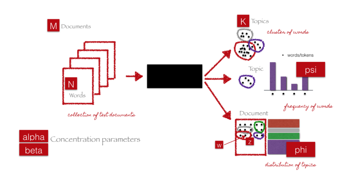
Because the topic model involves many concepts such as mathematics, we only introduce its use scheme here. Interested friends can read papers and other materials.

Generally, we will use LDA on TF-IDF or word frequency matrices. Finally, our results can also be disassembled into the following two core parts:

• Document topic matrix, which will be the characteristic matrix we need. What are you looking for.

• A topic term matrix that helps us look at potential topics in the corpus.

Here we use the above TDIDF matrix and set the subject to 2 for the experiment.

from sklearn.decomposition import LatentDirichletAllocation

lda       = LatentDirichletAllocation(n_components=2, max_iter=10000, random_state=0)
dt_matrix = lda.fit_transform(tfidf_matrix)
features  = pd.DataFrame(dt_matrix, columns=['T1', 'T2'])
features

	T1	T2
0	0.798663	0.201337
1	0.813139	0.186861
2	0.827378	0.172622
3	0.797794	0.202206

• View the topic and the contribution of each corresponding word.

tt_matrix = lda.components_
vocab = tfidf_model.get_feature_names()
for topic_weights in tt_matrix:
    topic = [(token, weight) for token, weight in zip(vocab, topic_weights)]
    topic = sorted(topic, key=lambda x: -x[1])
    topic = [item for item in topic if item[1] > 0.2]
    print(topic)
    print() 

[('the', 2.1446092537000254), ('sun', 1.7781565358915534), ('is', 1.7250615399950295), ('bright', 1.5425619519080085), ('sky', 1.3771748032988098), ('blue', 1.116020185537514), ('in', 0.9734645258594571), ('can', 0.828463031801155), ('see', 0.828463031801155), ('shining', 0.828463031801155), ('we', 0.828463031801155)]

[('can', 0.5461364394229279), ('see', 0.5461364394229279), ('shining', 0.5461364394229279), ('we', 0.5461364394229279), ('sun', 0.5440024650128295), ('the', 0.5434661558382532), ('blue', 0.5431709323301609), ('bright', 0.5404950589213404), ('sky', 0.5400833776748659), ('is', 0.539646632403921), ('in', 0.5307700509960934)]