Feature extraction - local features

Log, hog and dog differential operators are effective in detecting near circular spots

HOG characteristics

https://blog.csdn.net/coming_is_winter/article/details/72850511 https://blog.csdn.net/zouxy09/article/details/7929348/

Summary: Dalal Proposed Hog The process of feature extraction: the sample image is divided into several pixel units( cell)，The gradient direction is divided into 9 intervals( bin)，Histogram statistics of the gradient directions of all pixels in each direction interval are carried out in each unit to obtain a 9-dimensional feature vector, and each adjacent 4 units form a block( block)，The feature vectors in a block are connected to obtain a 36 dimensional feature vector. The sample image is scanned with a block with a scanning step of one unit. Finally, the features of all blocks are connected in series to obtain the features of human body.

For example, for 64*128 In terms of images, every 16*16 The pixels of form a cell，Every 2*2 individual cell Form a block because each cell There are 9 features, so there are 4 in each block*9=36 Features, in steps of 8 pixels, there will be 7 scanning windows in the horizontal direction and 15 scanning windows in the vertical direction. That is, 64*128 There are 36 pictures in total*7*15=3780 Two features.

Total number of features: one cell There are 9 features (9 gradient directions), and each feature cell There are in the block num*9 Features, step size, pixel specification: (column pixel number)-Step size)/step*(Row pixel number-Step size)/Step size,
Total feature number:(Column pixel number-Step size)/step*(Row pixel number-Step size)/step*num*9

LOG characteristics

The convolution operation between an image and a two-dimensional function is actually to obtain the similarity between the image and this function. Similarly, the convolution of image and Gaussian Laplace function is actually to obtain the similarity between image and Gaussian Laplace function. When the spot size in the image is close to the shape of Gaussian Laplacian function, the Laplacian response of the image reaches the maximum.

Laplace can be used to detect local extreme points in the image, but it is sensitive to noise. Therefore, before Laplace convolution of the image, we convolute the image with a Gaussian low-pass filter to remove the noise points in the image

Image first f(x,y)Using variance asσGaussian kernel for Gaussian filtering to remove noise in the image.

L(x,y;σ)=f(x,y)∗G(x,y;σ)
G(x,y;σ)Gaussian kernel
 Then, the Laplacian image of the image is:

∇^2=(∂^2L/∂^x2)+(∂^2L/∂y^2)
In fact, there is the following equation:

∇^2[G(x,y)∗f(x,y)]=∇^2[G(x,y)]∗f(x,y)

We can first find the Laplace operator of Gaussian kernel, and then convolute the image

Although using LoG can better detect the feature points in the image, it has too much computation. Usually, DoG (difference of Gaussian) can be used to approximate the LoG

Haar characteristics

Haar features are divided into three categories: edge features, linear features, center features and diagonal features, which are combined into feature templates. There are white and black rectangles in the feature template, and the feature value of the template is defined as < H3 > white rectangular pixels and subtracting the sum of black rectangular pixels</h3>

Haar like feature

https://blog.csdn.net/zouxy09/article/details/7929570

Integral graph is a fast algorithm that can calculate the sum of all regional pixels in the image only by traversing the image once, which greatly improves the efficiency of image eigenvalue calculation.

       The main idea of integral graph is to save the sum of pixels in the rectangular area formed by the image from the starting point to each point in memory as an array element. When calculating the sum of pixels in a certain area, you can directly index the elements of the array without recalculating the sum of pixels in this area, so as to speed up the calculation (this is called dynamic programming algorithm). The integral graph can use the same time (constant time) to calculate different features in multiple scales, so the detection speed is greatly improved.

       Let's see how it does it.

       Integral graph is a matrix representation method that can describe global information. The integral graph is constructed by position( i,j)Value at ii(i,j)Is the original image(i,j)Sum of all pixels in the upper left corner:

Normalized image

i¯(x,y)=(i(x,y)−μ)/cσ
In the formula i¯(x,y)Represents the normalized image, and i(x,y)Represents the original image, whereμRepresents the mean value of the image, andσRepresents the standard deviation of the image
σ2=(1/N)∑x2−μ2   2 Is square

SIFT feature

The full name of sift is Scale Invariant Feature Transform (people can recognize how an object rotates). SIFT feature is a very stable local feature, which maintains invariance to rotation, scale scaling, brightness change and so on.

There are four main steps

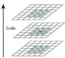
1. The extremum detection of scale space searches all images in scale space, and identifies the potential scale and selects the invariant points of interest through Gaussian differential function.

$L(x,y,σ)=G(x,y,σ)∗I(x,y)$

In order to effectively detect stable key points in scale space, Gaussian difference scale space is proposed( DOG scale-space). The image is convoluted by Gaussian difference kernel with different scales. Constructing Gaussian difference scale space(DOG scale-space): 

$D(x,y,σ)=(G(x,y,kσ)−G(x,y,σ))∗I(x,y)=L(x,y,kσ)−L(x,y,σ)$

σ Is the scale coordinate.σThe size determines the smoothness of the image, the large scale corresponds to the general features of the image, and the small scale corresponds to the detailed features of the image. BigσValue corresponds to rough scale(low resolution )，On the contrary, it corresponds to fine scale(high resolution). 

For an image I，It is established at different scales(scale)Image of,Each subsequent sample is 1 of the original image/4 Times.

Each point shall be compared with the points in the neighborhood and the points of upper and lower adjacent scales (9)+8+9)26 Compare points (to ensure that extreme points are detected in both scale space and two-dimensional image space). If a point is DOG When the maximum or minimum value is in the 26 fields of this layer and the upper and lower layers of the scale space, the point is considered to be a feature point of the image in this scale

1. Feature points are located at each candidate location, and the location scale is determined by a fitting fine model. The selection of key points is based on their stability.

Fitting three-dimensional quadratic function to accurately determine the location and scale of key points, and remove low contrast key points and unstable edge response points(because DoG The operator will produce strong edge response)，To enhance matching stability and anti noise ability

Test with Harris Corner Reference articles

1. The feature direction assignment is based on the local gradient direction of the image and assigned to one or more directions of each key point position. All subsequent operations are to transform the direction, scale and position of the key points, so as to provide the invariance of these features.

Each feature point calculates a direction, and further calculation is made according to this direction, *Using the gradient direction distribution characteristics of pixels in the neighborhood of key points, the direction parameters are specified for each key point, so that the operator has rotation invariance.

m(x,y)=(L(x+1,y)−L(x−1,y))2+(L(x,y+1)−L(x,y−1))2

√θ(x,y)=atan2(L(x,y+1)−L(x,y−1)L(x+1,y)−L(x−1,y)

Each key point has three information: location, scale and direction. Thus, a SIFT feature region can be determined.

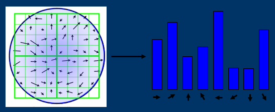
1. Feature points describe the local gradients of the image measured on the selected scale in the neighborhood around each feature point. These gradients are transformed into a representation, which allows relatively large local shape deformation and illumination transformation.

Gaussian function is the only feasible scale space kernel

scale space

Multiresolution image pyramid:

1. Smooth the original image
2. Downsampling the processed image (usually 1 in the horizontal and vertical directions)/2)After downsampling, a series of images are obtained. Obviously, in a traditional pyramid, the image of each layer is half the length and height of the image of the previous layer. Although the generation of multi-resolution image pyramid is simple, its essence is downsampling, and the local features of the image are difficult to maintain, that is, the scale invariance of the features cannot be maintained.

Gaussian scale space:

The blurring degree of the image is used to simulate the imaging process of the object on the retina when people are far from the object. The closer the object is, the larger the size is, the more blurred the image is. This is Gaussian scale space. Different parameters are used to blur the image (the resolution remains unchanged)

The image is convoluted with Gaussian function to blur the image. Images with different blur degrees can be obtained by using different "Gaussian kernel"

L(x,y,σ)=G(x,y,σ)∗I(x,y)

among G(x,y,σ)Gaussian kernel function
G(x,y,σ)=(1/2Πσ^2)e^((x^2+y^2)/(2σ^2))

The purpose of constructing scale space is to detect the feature points existing in different scales, and the better operator to detect the feature points is Δ^ 2g (Gauss Laplace, LoG)

DoG characteristics

Although using LoG can better detect the feature points in the image, it has too much computation. Usually, DoG (difference of Gaussian) can be used to approximate the LoG.

LOG can be regarded as an approximation of LOG, but it is more efficient than LOG. Let k be the scale factor of two adjacent Gaussian scale spaces, then the definition of DoG:

D(x,y,σ)=[G(x,y,kσ)−G(x,y,σ)]∗I(x,y)=L(x,y,kσ)−L(x,y,σ)

L(x,y, σ) Is the Gaussian scale space of the image The response image of DoG is obtained by subtracting the images of two adjacent Gaussian spaces

Harris corner feature extraction

< font color = Red > Harris corner detection is a first derivative matrix detection method based on image gray. The main idea of the detector is local self similarity / autocorrelation, that is, the similarity between the image block in a local window and the image block in the window after small movement in all directions</ font>

1. The corner can be the corner of two edges;

1. Corner points are characteristic points with two principal directions in the neighborhood;

The recognition of human eye diagonal points is usually completed in a local small area or small window. If the small window with this feature is moved in all directions and the gray level of the area in the window changes greatly, it is considered that corner points are encountered in the window. If the gray level of the image in the window does not change when the specific window moves in all directions of the image, there are no corners in the window; If the gray level of the image in the window changes greatly when the window moves in one direction, but does not change in other directions, the image in the window may be a straight line segment.

x^{y^z}=(1+{\rm e}^x)^{-2xy^w}

sqrt()

Conclusion: 1. Increase α It will reduce the corner response value R, reduce the flexibility of corner detection and reduce the number of detected corners; reduce α Value, which will increase the corner response value R, increase the sensitivity of corner detection and increase the number of detected corners.

1. Harris corner detection operator is insensitive to the changes of brightness and contrast
2. Harris corner detection operator has rotation invariance
3. Harris corner detection operator does not have scale invariance