Authors: Chen Yingxiang, Yang Zihan
Compilation: AI Youdao
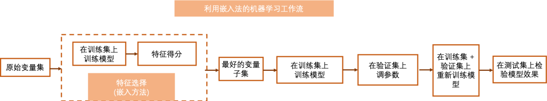
After data preprocessing, we generate a large number of new variables (for example, single hot coding generates a large number of variables containing only 0 or 1). But in fact, some newly generated variables may be redundant: on the one hand, they do not necessarily contain useful information, so they can not improve the performance of the model; On the other hand, these redundant variables will consume a lot of memory and computing power when building the model. Therefore, we should select features and select feature subsets for modeling.
Project address:
https://github.com/YC-Coder-Chen/feature-engineering-handbook/blob/master/%E4%B8%AD%E6%96%87%E7%89%88.md
This paper will introduce the Embedded Methods embedding method in feature engineering.
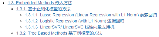
catalog:
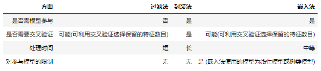
The feature selection process of filtering method is independent of the subsequent machine learning model, so filtering method may lead to poor model performance.
The encapsulation method uses a predefined supervised machine learning model to select the best function. However, because they need to train the model many times on a large number of possible feature subsets, although they usually lead to better performance, they also need longer processing time.
The embedded method embeds the feature selection process into the machine learning model, that is, machine learning is used to score each feature. The embedded method completes the selection of feature subset when creating the model. Therefore, they tend to have better performance than filtration. Compared with encapsulation methods, they save a lot of processing time and computing power.
A simple comparison of the three methods
1.3.1 method based on regularization model
Many machine learning models introduce regularization terms (L1 regularization or L2 regularization) into their loss functions to prevent over fitting problems. The L1 regular term in linear models (such as linear vector support machine, logistic regression, linear regression) can effectively reduce the characteristic coefficients of some features to zero, so as to realize the sparsity of solutions. Therefore, based on the characteristic coefficients of the linear model with regular terms, we can score the characteristics. The higher the coefficient, the more important this feature is in the linear model.
We can use the sklearn SelectFromModel function to delete features with low or zero feature coefficients.
1.3.1.1 Lasso Regression (Linear Regression with L1 Norm)
import numpy as np
from sklearn.feature_selection import SelectFromModel
from sklearn.linear_model import Lasso # We can also use ridge regression with L2 regular term


# Load dataset directly
from sklearn.datasets import fetch_california_housing
dataset = fetch_california_housing()
X, y = dataset.data, dataset.target # Using california_housing dataset to demonstrate


# Select the first 15000 observation points as the training set
# The rest are used as test sets
train_set = X[0:15000,:]
test_set = X[15000:,]
train_y = y[0:15000]


clf = Lasso(normalize=True, alpha = 0.001)
# Before linear regression, we need to scale the variables first, otherwise the regression coefficients cannot be compared
# Alpha controls the size of the regularization effect. The larger the alpha, the stronger the regularization effect


clf.fit(train_set, train_y) # Train on the training set
np.round(clf.coef_ ,3)
array([ 0.346, 0.003, -0. , -0. , -0. , -0. , -0.033, 0. ])
selector = SelectFromModel(clf, prefit=True, threshold=1e-5)
# The threshold is set to 1e-5, so features with absolute coefficients lower than 1e-5 will be deleted
# We can also set max_ The features parameter to select the first few most important features


transformed_train = selector.transform(train_set) # Transform training set
transformed_test = selector.transform(test_set) #Transform test set


assert np.array_equal(transformed_train, train_set[:,[0,1,6]])
# Select the first, second and seventh variables
assert np.array_equal(transformed_test, test_set[:,[0,1,6]])
1.3.1.2 Logistic Regression (with L1 Norm)
import numpy as np
from sklearn.feature_selection import SelectFromModel
from sklearn.linear_model import LogisticRegression
from sklearn.datasets import load_iris  # Using iris data as demonstration data set


# Load dataset
iris = load_iris()
X, y = iris.data, iris.target


# iris datasets need to be out of order before use
np.random.seed(1234)
idx = np.random.permutation(len(X))
X = X[idx]
y = y[idx]


# Select the first 100 observation points as the training set
# The remaining 50 observation points are used as the test set
train_set = X[0:100,:]
test_set = X[100:,]
train_y = y[0:100]


# Before performing logistic regression, we need to scale the variables first, otherwise the regression coefficients cannot be compared
from sklearn.preprocessing import StandardScaler
model = StandardScaler()
model.fit(train_set)
standardized_train = model.transform(train_set)
standardized_test = model.transform(test_set)


clf = LogisticRegression(penalty='l1', C = 0.7,
                         random_state=1234, solver='liblinear')
# We can also set the regular item to 'l2'
# C controls the size of the regularization effect. The larger C, the weaker the regularization effect


clf.fit(standardized_train, train_y)
np.round(clf.coef_,3)
array([[ 0. , 1. , -3.452, -0.159],
[ 0. , -1.201, 0.053, 0. ],
[ 0. , 0. , 1.331, 3.27 ]])selector = SelectFromModel(clf, prefit=True, threshold=1e-5) # The threshold is set to 1e-5, so features with absolute coefficients lower than 1e-5 will be deleted # We can also set max_ The features parameter to select the first few most important features transformed_train = selector.transform(train_set) # Transform training set transformed_test = selector.transform(test_set) #Transform test set assert np.array_equal(transformed_train, train_set[:,[1,2,3]]) # Select the second, third and fourth variables assert np.array_equal(transformed_test, test_set[:,[1,2,3]])
1.3.1.3 LinearSVR/ LinearSVC linear vector support machine
# LinearSVC is used to classify problems
# LinearSVR is used for regression problems
# Take LinearSVR as an example


import numpy as np
from sklearn.feature_selection import SelectFromModel
from sklearn.svm import LinearSVR


# Load dataset directly
from sklearn.datasets import fetch_california_housing
dataset = fetch_california_housing()
X, y = dataset.data, dataset.target # Using california_housing dataset to demonstrate


# Select the first 15000 observation points as the training set
# The rest are used as test sets
train_set = X[0:15000,:]
test_set = X[15000:,]
train_y = y[0:15000]


# Before performing logistic regression, we need to scale the variables first, otherwise the regression coefficients cannot be compared
from sklearn.preprocessing import StandardScaler
model = StandardScaler()
model.fit(train_set)
standardized_train = model.transform(train_set)
standardized_test = model.transform(test_set)


clf = LinearSVR(C = 0.0001, random_state = 123)
# C controls the size of the regularization effect. The larger C, the weaker the regularization effect


clf.fit(standardized_train, train_y)
np.round(clf.coef_,3)
array([ 0.254, 0.026, 0.026, -0.017, 0.032, -0.01 , -0.1 , -0.037])
selector = SelectFromModel(clf, prefit=True, threshold=1e-2)
# The threshold is set to 1e-2, so features with absolute coefficients lower than 1e-2 will be deleted
# We can also set max_ The features parameter to select the first few most important features


transformed_train = selector.transform(train_set) # Transform training set
transformed_test = selector.transform(test_set) #Transform test set


assert np.array_equal(transformed_train, train_set[:,[0,1,2,3,4,6,7]])
# Only the sixth variable is deleted
assert np.array_equal(transformed_test, test_set[:,[0,1,2,3,4,6,7]])
1.3.2 Tree Based Methods
A major branch of machine learning is tree based machine learning models, such as random forest, AdaBoost, Xgboost and so on. You can find more about these tree based machine learning models in a series of blogs written by my friends and me. Here:
https://github.com/YC-Coder-Chen/Tree-Math
These nonparametric tree models record how each variable gradually reduces the model loss in the bifurcation of tree nodes, and the feature importance of each feature can be analyzed according to the above records. We can delete some unimportant variables based on the importance of this characteristic.
# Let's take random forest as an example
import numpy as np
from sklearn.feature_selection import SelectFromModel
from sklearn.ensemble import RandomForestRegressor


# Load dataset directly
from sklearn.datasets import fetch_california_housing
dataset = fetch_california_housing()
X, y = dataset.data, dataset.target # Using california_housing dataset to demonstrate


# Select the first 15000 observation points as the training set
# The rest are used as test sets
train_set = X[0:15000,:]
test_set = X[15000:,]
train_y = y[0:15000]


# In the tree machine learning model, we do not need to scale variables


clf = RandomForestRegressor(n_estimators = 50, random_state = 123)


clf.fit(train_set, train_y)
np.round(clf.feature_importances_, 3)
array([0.52 , 0.045, 0.031, 0.026, 0.027, 0.139, 0.106, 0.107])
# Visual feature importance
import matplotlib.pyplot as plt
plt.rcParams['font.sans-serif']=['SimHei']
%matplotlib inline
importances = clf.feature_importances_
indices = np.argsort(importances)
plt.figure(figsize=(12,12))
plt.title('Characteristic importance')
plt.barh(range(len(indices)), importances[indices], color='seagreen', align='center')
plt.yticks(range(len(indices)),np.array(dataset.feature_names)[indices])
plt.xlabel('Relative importance of characteristics');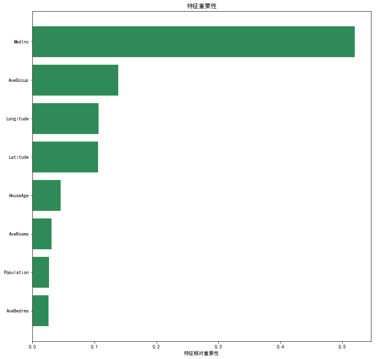
selector = SelectFromModel(clf, prefit=True, threshold='median')
# The threshold is set to 'median', that is, the median of feature importance is taken as the threshold, which is about 0.076
# We can also set max_ The features parameter to select the first few most important features


transformed_train = selector.transform(train_set)
transformed_test = selector.transform(test_set)
assert np.array_equal(transformed_train, train_set[:,[0,5,6,7]])
# Select the 1st, 6th, 7th and 8th features
assert np.array_equal(transformed_test, test_set[:,[0,5,6,7]])