Query analysis and tuning background
In the process of using the database, we often encounter the sudden slow down of SQL due to the following problems:
- Select wrong index
- Select the wrong connection order
- Range queries use different quick optimization strategies
- Execution method change of sub query selection
- Change of policy mode of semi connection selection
How to use the analysis tool OPTIMIZER TRACE to understand the optimization process and principle and to deeply analyze and tune slow SQL has become a powerful tool for advanced DBA s.
Let's first understand the overall process of query optimization:
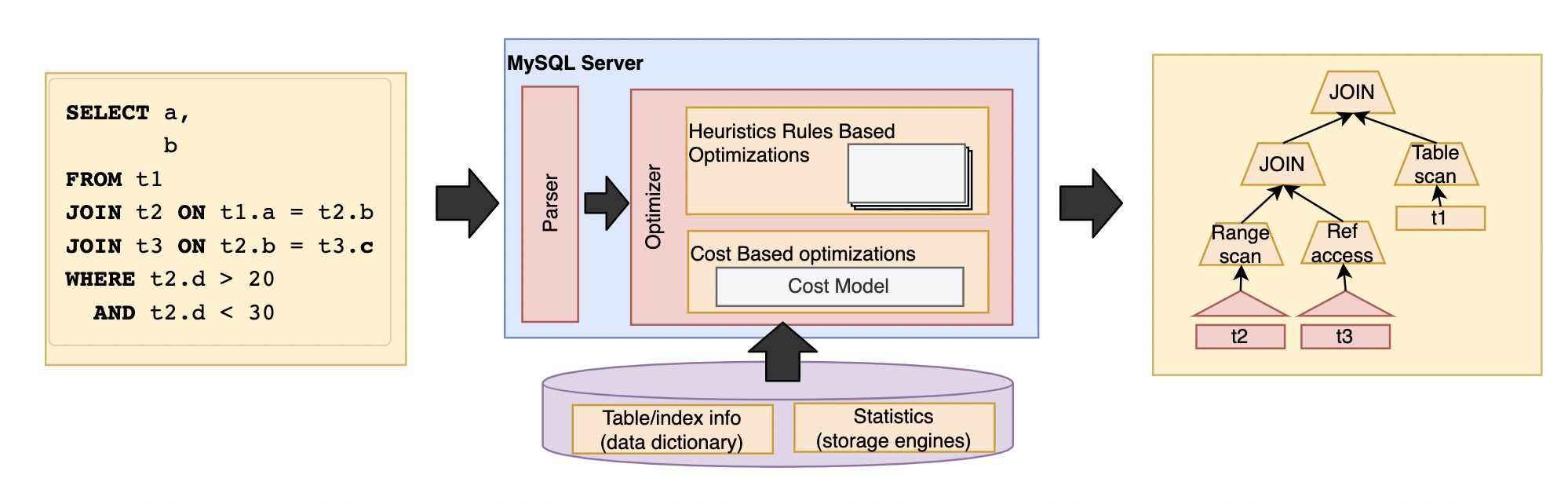
The main factors considered in this process are the access mode, connection sequence and method, and the execution strategy of semi connection and sub query. The main steps are:
- Calculate and set the cost of each operator
- Calculate and set the cost of partial or alternative execution plans
- Find the lowest cost execution plan
EXPLAIN tool
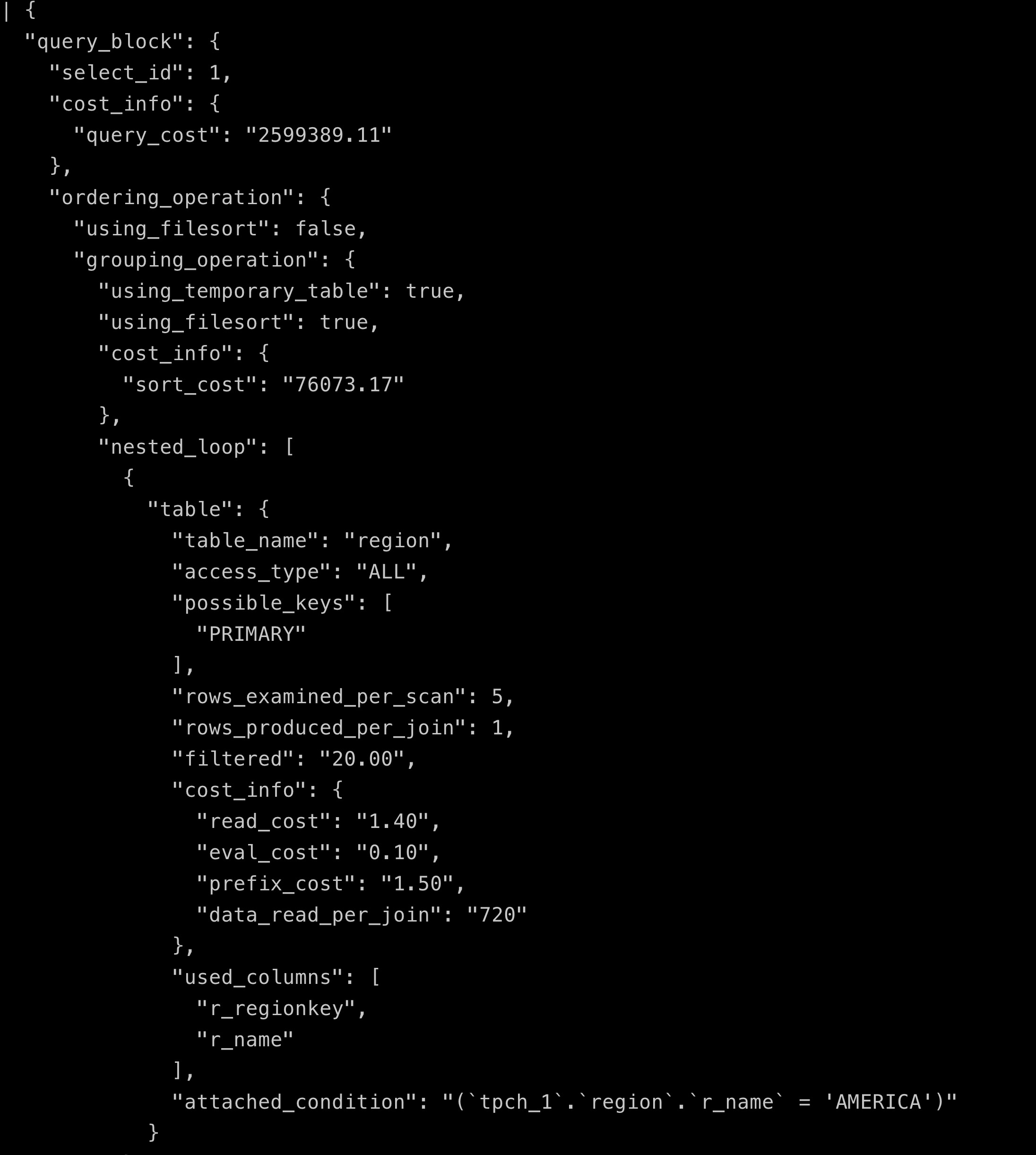
First, let's introduce the common explain tools. Explain is used to query the final execution plan and can be used through explain format=json see some specific cost information, such as TPCH Display of Q8 explain:
+----+-------------+----------+------------+--------+------------------------------------------------------------------+---------------+---------+-----------------------------+---------+----------+----------------------------------------------------+
| id | select_type | table    | partitions | type   | possible_keys                                                    | key           | key_len | ref                         | rows    | filtered | Extra                                              |
+----+-------------+----------+------------+--------+------------------------------------------------------------------+---------------+---------+-----------------------------+---------+----------+----------------------------------------------------+
|  1 | SIMPLE      | region   | NULL       | ALL    | PRIMARY                                                          | NULL          | NULL    | NULL                        |       5 |    20.00 | Using where; Using temporary; Using filesort       |
|  1 | SIMPLE      | n1       | NULL       | ref    | PRIMARY,i_n_regionkey                                            | i_n_regionkey | 5       | tpch_1.region.r_regionkey   |       5 |   100.00 | Using index                                        |
|  1 | SIMPLE      | orders   | NULL       | ALL    | PRIMARY,i_o_custkey,i_o_orderdate                                | NULL          | NULL    | NULL                        | 1488146 |    50.00 | Using where; Using join buffer (Block Nested Loop) |
|  1 | SIMPLE      | customer | NULL       | eq_ref | PRIMARY,i_c_nationkey                                            | PRIMARY       | 4       | tpch_1.orders.o_custkey     |       1 |     5.00 | Using where                                        |
|  1 | SIMPLE      | lineitem | NULL       | ref    | PRIMARY,i_l_orderkey,i_l_partkey,i_l_suppkey,i_l_partkey_suppkey | PRIMARY       | 4       | tpch_1.orders.o_orderkey    |       4 |   100.00 | Using where                                        |
|  1 | SIMPLE      | supplier | NULL       | eq_ref | PRIMARY,i_s_nationkey                                            | PRIMARY       | 4       | tpch_1.lineitem.l_suppkey   |       1 |   100.00 | Using where                                        |
|  1 | SIMPLE      | n2       | NULL       | eq_ref | PRIMARY                                                          | PRIMARY       | 4       | tpch_1.supplier.s_nationkey |       1 |   100.00 | NULL                                               |
|  1 | SIMPLE      | part     | NULL       | eq_ref | PRIMARY                                                          | PRIMARY       | 4       | tpch_1.lineitem.l_partkey   |       1 |    10.00 | Using where                                        |
+----+-------------+----------+------------+--------+------------------------------------------------------------------+---------------+---------+-----------------------------+---------+----------+----------------------------------------------------+
EXPLAIN format=json fragment display:
When looking at EXPLAIN, I mainly care about the following fields:
- id is query The serial number of the block, represented by the same number, and the table of the table field is in the same level query Block
- select_type usually refers to EXPLAIN_PRIMARY,EXPLAIN_SIMPLE,EXPLAIN_DERIVED,EXPLAIN_SUBQUERY,UNION,UNION_RESULT and MATERIALIZED represent the query Type of block
- Table is the table in the corresponding execution plan, or
- < derivedn >: the corresponding derived table, where N is select id, you can find the corresponding line from explain
- < subqueryn >: the corresponding materialized subquery. N is select id
- Partitions is a list of partitions that support pruning
- type refers to the access method, including the following content values. The performance is in order of system > const > eq_ref > ref > fulltext > ref_or_null > index_merge > unique_subquery > index_subquery > range > index > ALL
- System: the table has only one row (= system table). This is generally a variable value, which is a special case of const connection type.
- const: the largest matching row in the table, which will be read at the beginning of the query. Because there is only one row, the column values in this row can be considered constant by the rest of the optimizer. const is used to compare primary with constant values All parts of the key or unique index.
- eq_ref: for each row combination from the previous table, read one row from the table. This is probably the best join type, except const. It is used to join all parts of an index, and the index is UNIQUE or PRIMARY KEY. eq_ref can be used to= The indexed column that the operator compares. The comparison value can be a constant or an expression that uses the columns of the table read before the table.
- Ref: for each row combination from the previous table, all rows with matching index values are read from this table. If the join uses only the leftmost prefix of the KEY, or if the KEY is not UNIQUE or PRIMARY KEY (in other words, if the join cannot select a single row based on the keyword), ref is used. This join type is good if the KEY used matches only a few rows. Ref can be used for indexed columns using the = or < = > operators.
- ref_or_null: the join type is like ref, but MySQL is added to search for rows containing NULL values. Optimization of this join type is often used in solving subqueries.
- index_merge: this join type indicates that the index merge optimization method is used. In this case, the key column contains a list of the indexes used, key_len contains the longest key element of the index used.
- unique_subquery: this type replaces ref: value of in subquery in the following form IN (SELECT primary_key FROMsingle_table WHERE some_expr);unique_subquery is an index lookup function that can completely replace subqueries and is more efficient.
- index_subquery: this join type is similar to unique_subquery. You can replace the in subquery, but only for non unique indexes in the following form of subquery: value IN SELECT key_column FROM single_table WHERE some_expr)
- Range: retrieve only rows IN a given range, using an index to select rows. The key column shows which index IS used. key_len contains the longest key element of the index used. The ref column IS NULL IN this type. When =, < >, >, > =, <, < =, IS NULL, < = >, BETWEEN or IN operators. When comparing keyword columns with constants, you can use range
- Index: the join type is the same as ALL, except that only the index tree is scanned. This is usually faster than ALL because the index file is usually smaller than the data file.
- All: perform a complete table scan for each row combination from the previous table. This is usually bad if the table is the first table that is not marked const, and it is usually bad in its case. Generally, more indexes can be added instead of all, so that rows can be retrieved based on constant values or column values in the previous table.
- The extra field contains more information, including whether to use a temporary table Temporary), whether to use file sorting filesort), whether to use where filtering Where or Using under index conditions index condition), whether to use connection buffer join Buffer), whether to inform that there are no rows that meet the conditions (Impossible) Where), or Using an index Index), because this article focuses on optimizer trace, I won't explain it in detail here.
In the latest version 8.0.18, format=tree is added to better see the execution process of the new iterator, as follows:
| -> Sort: all_nations.o_year                                                                                                                                                                           -> Table scan on <temporary>
        -> Aggregate using temporary table
            -> Nested loop inner join  (cost=9.91 rows=1)
                -> Nested loop inner join  (cost=8.81 rows=1)
                    -> Nested loop inner join  (cost=7.71 rows=1)
                        -> Nested loop inner join  (cost=6.61 rows=1)
                            -> Nested loop inner join  (cost=5.51 rows=1)
                                -> Nested loop inner join  (cost=4.41 rows=1)
                                    -> Nested loop inner join  (cost=3.31 rows=1)
                                        -> Filter: (orders.o_custkey is not null)  (cost=2.21 rows=1)
                                            -> Index range scan on orders using i_o_orderdate, with index condition: (orders.o_orderDATE between DATE'1995-01-01' and DATE'1996-12-31')  (cost=2.21 rows=1)
                                        -> Filter: (customer.c_nationkey is not null)  (cost=1.10 rows=1)
                                            -> Single-row index lookup on customer using PRIMARY (c_custkey=orders.o_custkey)  (cost=1.10 rows=1)
                                    -> Filter: (n1.n_regionkey is not null)  (cost=1.10 rows=1)
                                        -> Single-row index lookup on n1 using PRIMARY (n_nationkey=customer.c_nationkey)  (cost=1.10 rows=1)
                                -> Filter: (region.r_name = 'AMERICA')  (cost=1.10 rows=1)
                                    -> Single-row index lookup on region using PRIMARY (r_regionkey=n1.n_regionkey)  (cost=1.10 rows=1)
                            -> Filter: ((lineitem.l_suppkey is not null) and (lineitem.l_partkey is not null))  (cost=1.10 rows=1)
                                -> Index lookup on lineitem using PRIMARY (l_orderkey=orders.o_orderkey)  (cost=1.10 rows=1)
                        -> Filter: (supplier.s_nationkey is not null)  (cost=1.10 rows=1)
                            -> Single-row index lookup on supplier using PRIMARY (s_suppkey=lineitem.l_suppkey)  (cost=1.10 rows=1)
                    -> Single-row index lookup on n2 using PRIMARY (n_nationkey=supplier.s_nationkey)  (cost=1.10 rows=1)
                -> Filter: (part.p_type = 'ECONOMY ANODIZED STEEL')  (cost=1.10 rows=1)
                    -> Single-row index lookup on part using PRIMARY (p_partkey=lineitem.l_partkey)  (cost=1.10 rows=1)
 |
EXPLAIN shows what the final execution plan looks like. It can be used to analyze whether a new index needs to be created, or compare the previous execution plan to determine whether there are performance problems caused by changes, but it is impossible to know more deeply how the optimizer selects the final plan from many available methods.
OPTIMIZER TRACE
EXPLAIN shows the result of selection, so for DBA s who want to know why to execute like this, OPTIMIZER TRACE is to show why the execution plan is accessed
How to generate OPTIMIZER TRACE
SET optimizer_trace = "enabled=on";
SET optimizer_trace_max_mem_size=655350;
<SQL>
SELECT trace FROM information_schema.optimizer_trace
INTO OUTFILE <filename> LINES TERMINATED BY '';
#  perhaps
SELECT trace FROM information_schema.optimizer_trace \G
SET optimizer_trace ="enabled=off";
For example:
test:tpch_1> SELECT * FROM information_schema.`OPTIMIZER_TRACE`\G
*************************** 1. row ***************************
                            QUERY: select         o_year,         sum(case                 when nation = 'BRAZIL' then volume                 else 0         end) / sum(volume) as mkt_share from
      (                 select                         extract(year from o_orderdate) as o_year,                         l_extendedprice * (1 - l_discount) as volume,                         n2.n_
name as nation                 from                         part,                         supplier,                         lineitem,                         orders,                         custom
er,                         nation n1,                         nation n2,                         region                 where                         p_partkey = l_partkey
 and s_suppkey = l_suppkey                         and l_orderkey = o_orderkey                         and o_custkey = c_custkey                         and c_nationkey = n1.n_nationkey
              and n1.n_regionkey = r_regionkey                         and r_name = 'AMERICA'                         and s_nationkey = n2.n_nationkey                         and o_orderdate betwe
en date '1995-01-01' and date '1996-12-31'                         and p_type = 'ECONOMY ANODIZED STEEL'         ) as all_nations group by         o_year order by         o_year
                            TRACE: {
  "steps": [
    {
      "join_preparation": {
        "select#": 1,
        "steps": [
          {
            "join_preparation": {
              "select#": 2,
              "steps": [
                {
                  "expanded_query": "/* select#2 */ select extract(year from `orders`.`o_orderDATE`) AS `o_year`,(`lineitem`.`l_extendedprice` * (1 - `lineitem`.`l_discount`)) AS `volume`,`n2`.`n_
name` AS `nation` from `part` join `supplier` join `lineitem` join `orders` join `customer` join `nation` `n1` join `nation` `n2` join `region` where ((`part`.`p_partkey` = `lineitem`.`l_partkey`)
 and (`supplier`.`s_suppkey` = `lineitem`.`l_suppkey`) and (`lineitem`.`l_orderkey` = `orders`.`o_orderkey`) and (`orders`.`o_custkey` = `customer`.`c_custkey`) and (`customer`.`c_nationkey` = `n1
`.`n_nationkey`) and (`n1`.`n_regionkey` = `region`.`r_regionkey`) and (`region`.`r_name` = 'AMERICA') and (`supplier`.`s_nationkey` = `n2`.`n_nationkey`) and (`orders`.`o_orderDATE` between DATE'
1995-01-01' and DATE'1996-12-31') and (`part`.`p_type` = 'ECONOMY ANODIZED STEEL'))"
                }
              ]
            }
          },
          {
            "derived": {
              "table": "``.`` `all_nations`",
              "select#": 2,
              "merged": true
            }
          },
......

MISSING_BYTES_BEYOND_MAX_MEM_SIZE: 801464
          INSUFFICIENT_PRIVILEGES: 0
1 row in set (0.10 sec)
Because the optimization process may output a lot, if a certain limit is exceeded, the redundant text will not be displayed. This field shows the number of text bytes ignored_ BYTES_ BEYOND_ MAX_ MEM_ If the size is not 0, it means that the Trace is truncated and needs to be reset to a larger value, optimizer_trace_max_mem_size, such as 1000000 > 801464.
You can also use the JSON browser plug-in to display Trace, which is more intuitive
OPTIMIZER The structure of TRACE is divided into three categories:
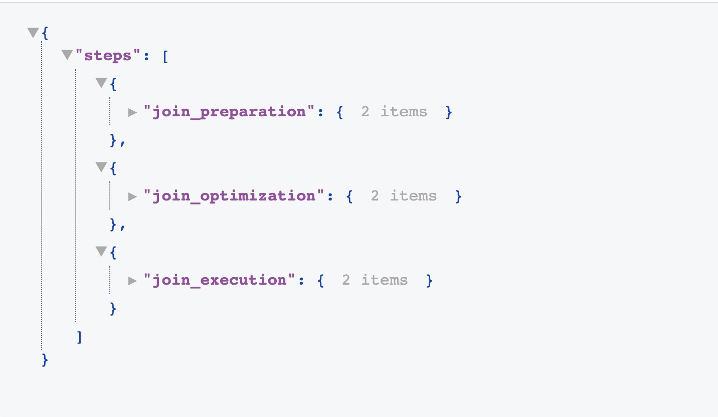
OPTIMIZER TRACE analysis
Optimizer Trace tracks the overall process of the optimizer and the actuator. As shown in the figure, the overall flow chart of the optimizer and the scope of trace collection are shown
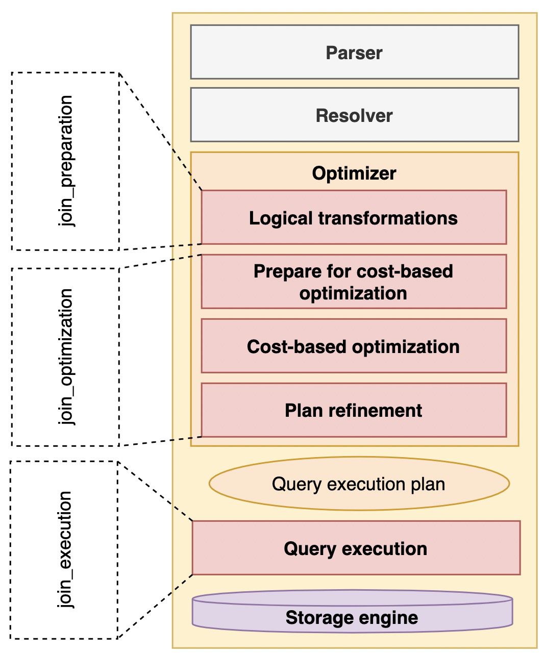
join_preparation stage display
We can know that in the preparation stage of SQL, semantic parsing, syntax detection and permanent rule-based transformation are mainly done, including the transformation from external connection to internal connection, merging views or derived tables and some sub query transformation. For details, please refer to paoding jieniu - diagram mysql 8.0 optimizer query analysis chapter and paoding jieniu - Graphical MySQL 8.0 optimizer query transformation. Now let's observe the embodiment of several typical conversion processes in trace.
Derived Merge rule conversion
{
  "derived": {
    "table": "``.`` `all_nations`",
    "select#": 2,
    "merged": true
  }
},
Convert external connection to internal connection rule set outer_join_to_inner_join,JOIN_condition_to_WHERE and parentthesis_ removal
{
  "join_preparation": {
    "select#": 1,
      "steps": [
        {
          "expanded_query": "/* select#1 */ select `orders`.`o_orderkey` AS `o_orderkey` from (`orders` left join `lineitem` on((`order
          s`.`o_orderkey` = `lineitem`.`l_orderkey`))) where (`lineitem`.`l_discount` > 0.10)"
          },
          {
            "transformations_to_nested_joins": {
              "transformations": [
                "outer_join_to_inner_join",
                "JOIN_condition_to_WHERE",
                "parenthesis_removal"
              ],
              "expanded_query": "/* select#1 */ select `orders`.`o_orderkey` AS `o_orderkey` from `orders` join `lineitem` where ((`linei
          tem`.`l_discount` > 0.10) and (`orders`.`o_orderkey` = `lineitem`.`l_orderkey`))"
            }
          }
        ]
      }
IN 8.0.16, convert EXISTS subquery to IN subquery rule:
SELECT o_orderpriority, COUNT(*) AS order_count FROM orders WHERE EXISTS (SELECT * FROM lineitem WHERE l_orderkey =
o_orderkey AND l_commitdate < l_receiptdate) GROUP BY o_orderpriority ORDER BY o_orderpriority;

{                                                                                                                   [642/44613]
 "transformation": {
   "select#": 2,
     "from": "IN (SELECT)",
       "to": "semijoin",
         "chosen": true,
           "transformation_to_semi_join": {
             "subquery_predicate": "exists(/* select#2 */ select 1 from `lineitem` where ((`lineitem`.`l_orderkey` = `orders`.`o_order
             key`) and (`lineitem`.`l_commitDATE` < `lineitem`.`l_receiptDATE`)))",
                "embedded in": "WHERE",
                "evaluating_constant_semijoin_conditions": [
                ],
                "semi-join condition": "((`lineitem`.`l_commitDATE` < `lineitem`.`l_receiptDATE`) and (`orders`.`o_orderkey` = `lineitem`
.`l_orderkey`))",
                "decorrelated_predicates": [
                  {
                    "outer": "`orders`.`o_orderkey`",
                    "inner": "`lineitem`.`l_orderkey`"
                  }
                ]
              }
            }
          },
          {
            "transformations_to_nested_joins": {
              "transformations": [
                "semijoin"
              ],
              "expanded_query": "/* select#1 */ select `orders`.`o_orderpriority` AS `o_orderpriority`,count(0) AS `order_count` from `o
              rders` semi join (`lineitem`) where ((`lineitem`.`l_commitDATE` < `lineitem`.`l_receiptDATE`) and (`orders`.`o_orderkey` = `lineitem`.`l_orderkey`)) group by `orders`.`o_orderpriority` order by `orders`.`o_orderpriority`"                                                               }
          }
join_optimization presentation
In addition to making some subsequent logical transformations in prepare, this stage mainly shows the cost based optimization process of the optimizer, including access methods, connection methods and sequences, as well as some specific optimizations for execution plans. However, it will also solve some legacy logical conversion rules, such as NOT elimination, equivalence transfer, constant calculation and condition removal.
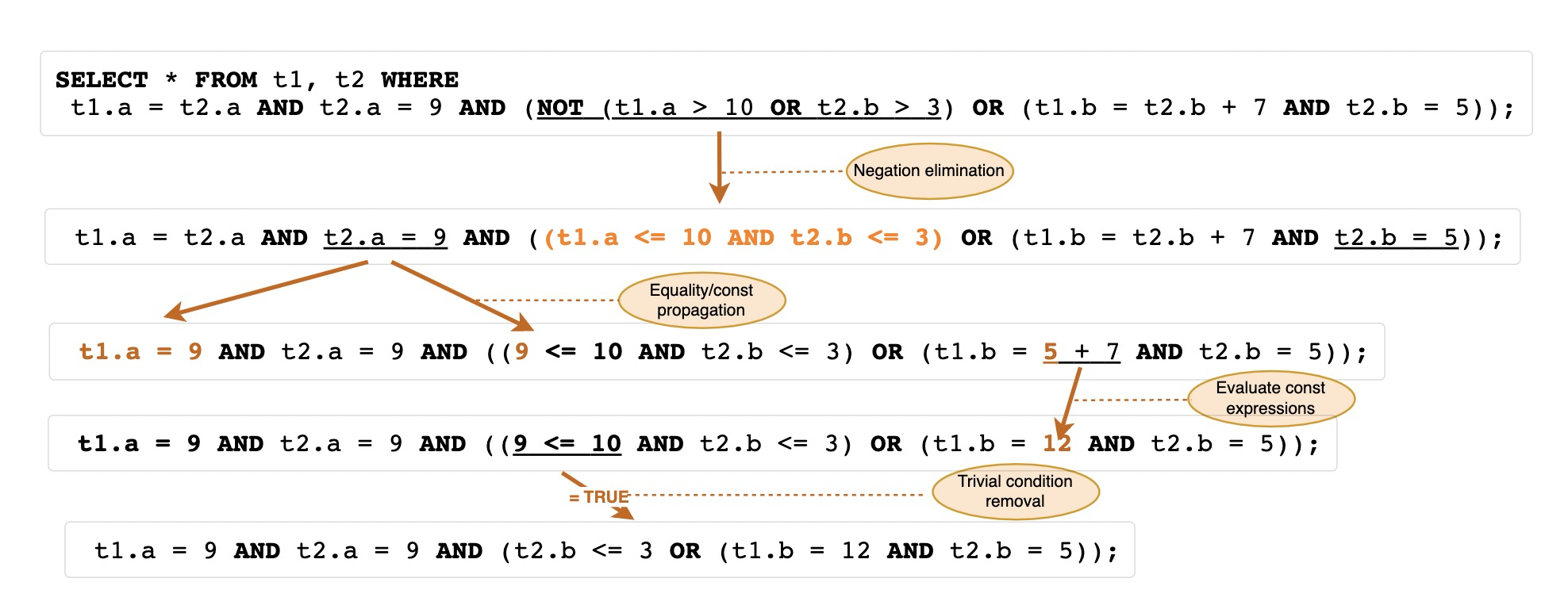
You can see the trace as follows:
    {                                                                                                                        [174/44947]
      "join_optimization": {
        "select#": 1,
        "steps": [
          {
            "condition_processing": {
              "condition": "WHERE",
              "original_condition": "((`t1`.`a` = `t2`.`a`) and (`t2`.`a` = 9) and (((`t1`.`a` <= 10) and (`t2`.`b` <= 3)) or ((`t1`.`b`
 = (`t2`.`b` + 7)) and (`t2`.`b` = 5))))",
              "steps": [
                {
                  "transformation": "equality_propagation",
                  "resulting_condition": "((((9 <= 10) and (`t2`.`b` <= 3)) or ((`t1`.`b` = (5 + 7)) and multiple equal(5, `t2`.`b`))) a
nd multiple equal(9, `t1`.`a`, `t2`.`a`))"
                },
                {
                  "transformation": "constant_propagation",
                  "resulting_condition": "((((9 <= 10) and (`t2`.`b` <= 3)) or ((`t1`.`b` = 12) and multiple equal(5, `t2`.`b`))) and mu
ltiple equal(9, `t1`.`a`, `t2`.`a`))"
                },
                {
                  "transformation": "trivial_condition_removal",
                  "resulting_condition": "(((`t2`.`b` <= 3) or ((`t1`.`b` = 12) and multiple equal(5, `t2`.`b`))) and multiple equal(9,
`t1`.`a`, `t2`.`a`))"
                }
              ]
            }
          },
Let's use trace to unlock the mystery of cost based access, that is, access mode, connection method and order, whether to use connection buffer and sub query strategy, etc.
Table access mode selection
First, the cost of Table access is estimated, which is mainly divided into Table Scan (full Table scan), index Look Up (ref) access method, index Scan (index scan), range Index Scan (index range query) and some alternative Quick Range Scan (fast range access mode). Each classification can be calculated independently to select the best scheme, and finally select the lowest cost access mode among all types of best schemes.
- Analyze dependencies between tables
- Table: the name of the table involved. If there is an alias, it will also be displayed
- row_may_be_null: whether the row can be NULL. This refers to whether the data in this table can be NULL after the JOIN operation. If LEFT is used in the statement JOIN, then the row of the next table_ may_ be_ NULL will be displayed as true
- map_bit: the mapping number of the table, increasing from 0
- depends_on_map_bits: dependent mapping table. Mainly when using STRAIGHT_JOIN forcibly controls the connection sequence or LEFT JOIN/RIGHT If the join order is different, it will be displayed in dependencies_ on_ map_ The map of the preceding table is displayed in bits_ Bit value.
{
  "table_dependencies": [
    {
      "table": "`part`",
      "row_may_be_null": false,
      "map_bit": 0,
      "depends_on_map_bits": []
    },
    {
    "table": "`supplier`",
    "row_may_be_null": false,
    "map_bit": 1,
    "depends_on_map_bits": []
    },
    ......
    ]
},- Lists the indexes of all available ref types
The optimizer first passes Ref_ optimizer_ key_ Use step to view the ref index that can be used by each table in SQL for subsequent calculation of access and connection costs. Ref is a method that must be equivalent comparison. It is usually used in single table conditions and multi table connection conditions.
{
  "ref_optimizer_key_uses": [
    {
    "table": "`part`",
    "field": "p_partkey",
    "equals": "`lineitem`.`l_partkey`",
    "null_rejecting": true
    },
    {
    "table": "`supplier`",
    "field": "s_suppkey",
    "equals": "`lineitem`.`l_suppkey`",
    "null_rejecting": true
    },
    ......
    {
    "table": "`region`",
    "field": "r_regionkey",
    "equals": "`n1`.`n_regionkey`",
    "null_rejecting": true
    }
  ]
},
Next, traverse each table to evaluate the cost of access mode
- Cost evaluation of full table scanning
{
  "table": "`orders`",
  "range_analysis": {
    "table_scan": {
    "rows": 1488146,
    "cost": 151868,
    "in_memory": 1
  },
......
in_memory is a newly added parameter in xxx version. It is used to calculate the cost of accessing data. page is not in memory but on disk. 1 means that the data is in memory.
- Overlay index scan estimation
best_covering_index_scan: if there is an overlay index, list the overlay index
 select max(l_shipdate), sum(l_shipdate) from lineitem where l_shipdate <= date '1998-12-01' - interval '90' day;
"range_analysis": {
  "table_scan": {
    "rows": 1497730,
    "cost": 150488
  },
......
"best_covering_index_scan": {
  "index": "i_l_shipdate",
    "cost": 151967,
    "chosen": false,
    "cause": "cost"
},
It can be clearly seen that there is coverage index in time. Due to weak filtering, the cost of full table scanning is similar to that of coverage index, so full table scanning is selected.
- Evaluation and optimization of range index scanning and fast index scanning
It can be clearly seen that first, list the potential_range_indexes of the table that can be scanned by RANGE. Here, it will directly determine whether it can be considered, "usable" represents whether it can be used, and "cause" represents the reason for rejection.
Next, start to check whether there is a Quick range lookup method (Quick) Range Scan), such as group_index_range and skip_scan_range, etc. "chosen" represents whether the Quick access method is used, and "cause" is the reason for rejection. The example SQL shown here is rejected because it is not a single table. If it can be used, the reason for rejection is cost.
SELECT a, b FROM t1 GROUP BY a, b;
SELECT DISTINCT a, b FROM t1;
SELECT a, MIN(b) FROM t1 GROUP BY a;
At this time, we have selected the best access method (Table) according to cost Scan vs Quick Range Scan). Next, let's continue to view the range Index separately Range Scan) whether there is the most available scheme, and these possible options are placed in the range_ scan_ In alternatives, we can see whether the specific Index used and the source of Index estimation cost (dive, statistics, histogram, etc.) use some special optimization modes (rowid_ordered, using_mrr, index_only), and the proportion of memory occupied by the Index. "chosen" means whether the quick access method is used, and "cause" is the reason for being rejected. We usually see that cost is pruned off.
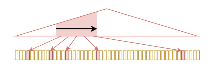
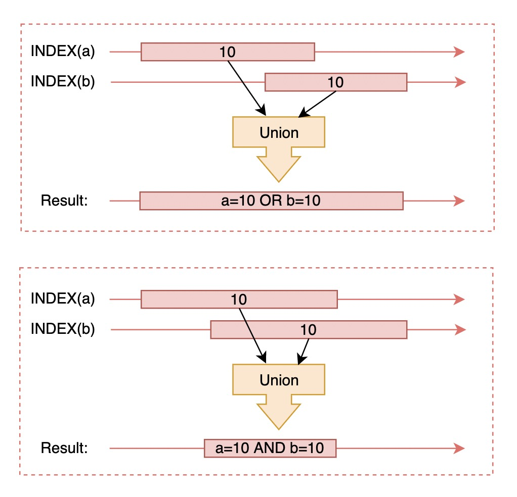
Previously, we estimated the cost of table access for an index. In fact, there is another fast access method based on the common method of multiple indexes, that is, through row The access method of intersection and union after ids sorting will be placed in analyzing_ roworder_ In intersect. "usable" stands for whether it may be used, and "cause" stands for the reason for rejection. Usually we get too_ few_ roworder_ The reason for scans.
"analyzing_index_merge_union": [
  {
    "indexes_to_merge": [
      {
        "range_scan_alternatives": [
          {
            "index": "ind1",
            "ranges": [
              "2 <= key1_part1 <= 2"
            ],
            "index_dives_for_eq_ranges": true,
            "rowid_ordered": false,
            "using_mrr": false,
            "index_only": true,
            "rows": 1,
            "cost": 0.36,
            "chosen": true
          }
        ],
        "index_to_merge": "ind1",
        "cumulated_cost": 0.36
      },
      {
        "range_scan_alternatives": [
          {
            "index": "ind2",
            "ranges": [
              "4 <= key2_part1 <= 4"
            ],
            "index_dives_for_eq_ranges": true,
            "rowid_ordered": false,
            "using_mrr": false,
            "index_only": true,
            "rows": 1,
            "cost": 0.36,
            "chosen": true
          }
        ],
        "index_to_merge": "ind2",
        "cumulated_cost": 0.72
      }
    ],
    "cost_of_reading_ranges": 0.72,
    "cost_sort_rowid_and_read_disk": 0.4375,
    "cost_duplicate_removal": 0.254503,
    "total_cost": 1.412
  },
  "chosen_range_access_summary": {
    "range_access_plan": {
    "type": "index_merge",
    "index_merge_of": [
      {
        "type": "range_scan",
        "index": "ind1",
        "rows": 1,
        "ranges": [
          "2 <= key1_part1 <= 2"
        ]
      },
      {
        "type": "range_scan",
          "index": "ind2",
          "rows": 1,
          "ranges": [
             "4 <= key2_part1 <= 4"
          ]
      }
    ]
  },
  "rows_for_plan": 2,
  "cost_for_plan": 1.412,
  "chosen": true
}
If the selected range scanning mode is selected in the whole range analysis process, you can see chosen_range_access_summary attribute, otherwise there is no.
- rows_for_plan: the number of scan lines of the execution plan
- cost_for_plan: the execution cost of the execution plan
- chosen: select this execution plan
"chosen_range_access_summary": {
  "range_access_plan": {
    "type": "range_scan",
      "index": "i_l_shipdate",
        "rows": 1,
          "ranges": [
            "NULL < l_shipDATE <= 0x229d0f"
          ]
  },
  "rows_for_plan": 1,
  "cost_for_plan": 0.61,
  "chosen": true
}- Select the optimal execution plan (considered_execution_plans)
Now comes the stage of considering the final execution plan, which is responsible for comparing the cost of each feasible plan and selecting the relatively optimal execution plan. In the single table scenario, only the access methods (Ref) of Range and ref will be considered access vs. table/index scan).
"considered_execution_plans": [                                                                                   [52/47176]
{                                                                                                               [58/47542]
  "plan_prefix": [
  ],
  "table": "`lineitem`",
    "best_access_path": {
      "considered_access_paths": [
        {
          "access_type": "ref",
          "index": "i_l_partkey",
          "rows": 1,
          "cost": 0.35,
          "chosen": true
        },
        {
          "access_type": "ref",
          "index": "i_l_partkey_suppkey",
          "rows": 1,
          "cost": 0.35,
          "chosen": false
        },
        {
          "access_type": "range",
          "range_details": {
            "used_index": "i_l_partkey"
          },
          "chosen": false,
          "cause": "heuristic_index_cheaper"
        }
      ]
    },
If greedy algorithm is required for multiple tables, select the most common connection order and method. The more important attributes are:
- plan_prefix: the pre execution plan of the current plan.
- Table: the name of the table involved. If there is an alias, it will also be displayed
- best_access_path: table access cost of this layer
- condition_filtering_pct: similar to the filtered column, it is an estimated value
- rows_for_plan: the number of final scan lines of the execution plan, which is considered by_ access_ paths.rows X condition_ filtering_ Obtained by PCT calculation.
- cost_for_plan: the cost of executing the plan, which is considered by_ access_ Paths.cost is obtained by adding
- chosen: is the execution plan selected
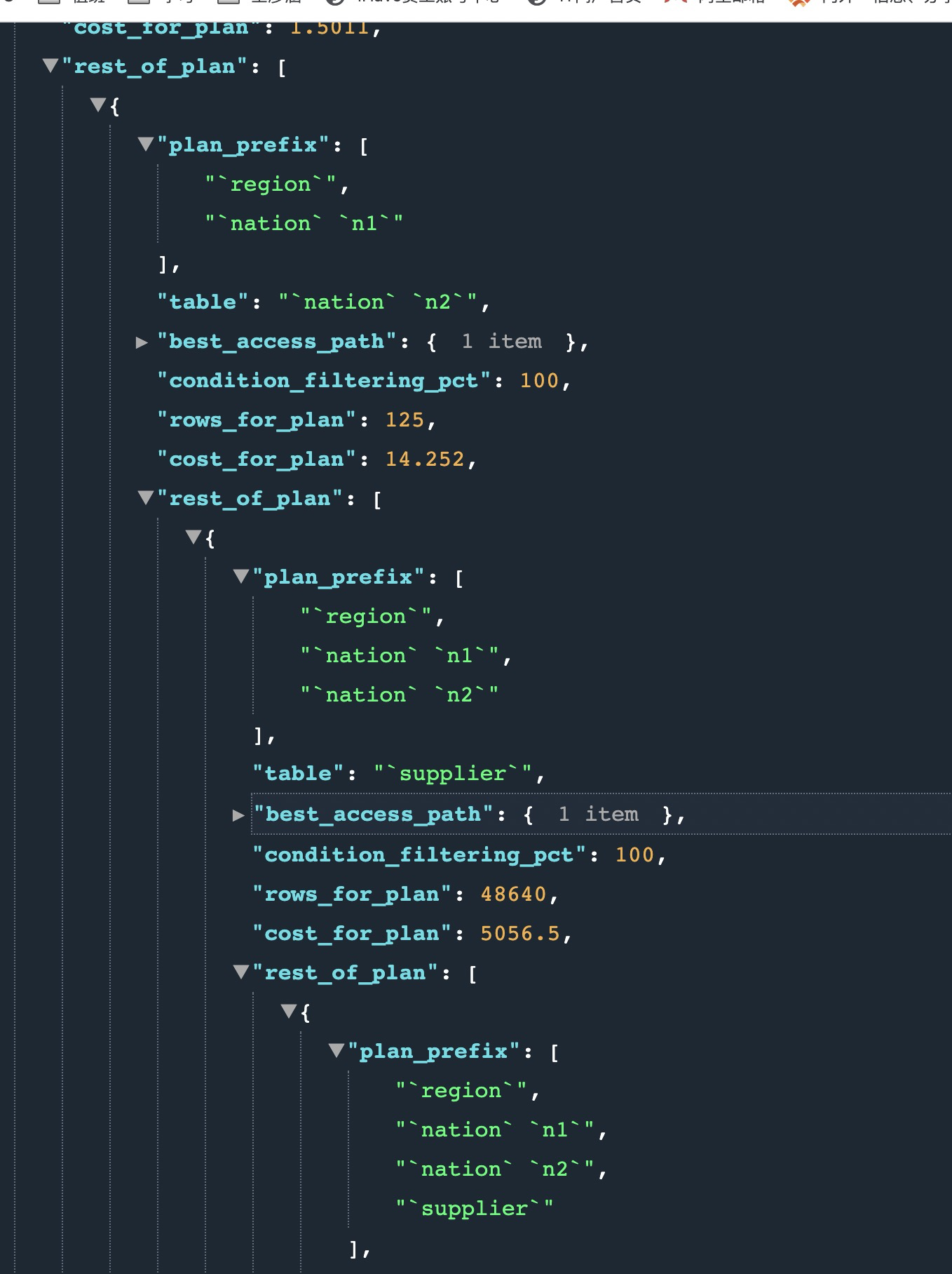
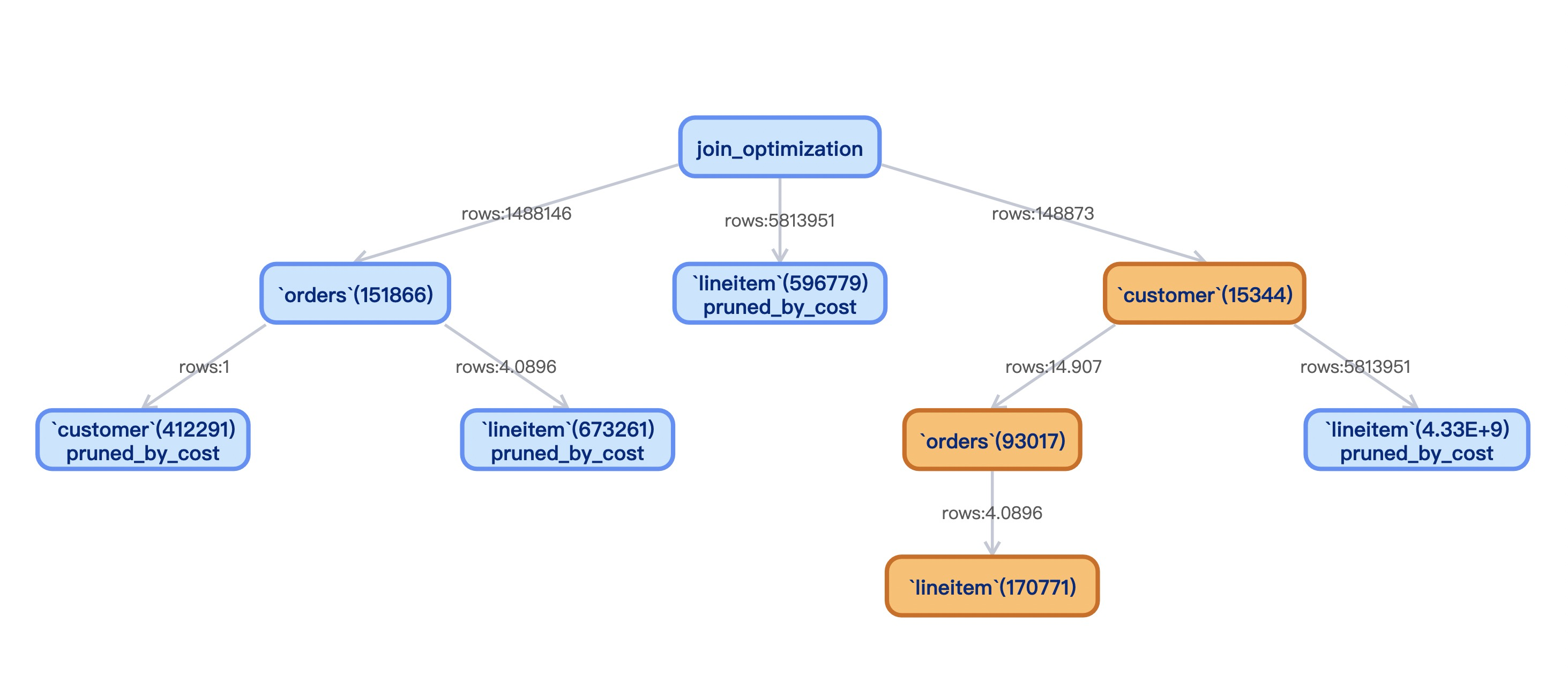
Let's take a complete look through the tree. Orange is the order of the final selected JOIN. customer, orders and lineitem:
- Consideration of other factors of access and connection
- Join buffering (BNL/BKA/HASH JOIN)
"rest_of_plan": [
  {
    "plan_prefix": [
      "`t1`"
    ],
    "table": "`t2`",
    "best_access_path": {
      "considered_access_paths": [
        {
          "rows_to_scan": 5,
          "filtering_effect": [
          ],
          "final_filtering_effect": 0.3333,
          "access_type": "scan",
          "using_join_cache": true,
          "buffers_needed": 1,
          "resulting_rows": 1.6665,
          "cost": 0.75002,
          "chosen": true
        }
      ]
    },
    "condition_filtering_pct": 60.006,
    "rows_for_plan": 1,
    "cost_for_plan": 1.30002,
    "chosen": true
  }
]- Filtering effects of conditions
If the where condition in conditional filtering is not in the index condition and there are table connections, you can also focus on filtering_ The value of effect through set optimizer_switch="condition_fanout_filter=on"; You can turn off the optimization.
  "table": "`employee`",
  "best_access_path": {
    "considered_access_paths": [
      {
        "rows_to_scan": 10,
        "filtering_effect": [
        ],
        "final_filtering_effect": 0.1,
        "access_type": "scan",
        "resulting_rows": 1,
        "cost": 1.75,
        "chosen": true
      }
    ]
  },
By doing additional where Condition filtering on the driver table Filtering), which can limit the driving table to a smaller range, so that the optimizer can make a better execution plan.
root:test> set optimizer_switch="condition_fanout_filter=on";
Query OK, 0 rows affected (0.00 sec)

root:test> explain SELECT *   FROM employee JOIN department ON employee.dept_id = department.DNO   WHERE employee.emp_name = 'John'   AND employee.hire_date BETWEEN '2018-01-01' AND '2018-06-01';
+----+-------------+------------+----------------------+--------+---------------+---------+---------+-----------------------+------+----------+-------------+
| id | select_type | table      | partitions           | type   | possible_keys | key     | key_len | ref                   | rows | filtered | Extra       |
+----+-------------+------------+----------------------+--------+---------------+---------+---------+-----------------------+------+----------+-------------+
|  1 | SIMPLE      | employee   | p_1000,p_2000,p_3000 | ALL    | NULL          | NULL    | NULL    | NULL                  |   10 |    10.00 | Using where |
|  1 | SIMPLE      | department | NULL                 | eq_ref | PRIMARY       | PRIMARY | 4       | test.employee.dept_id |    1 |   100.00 | Using where |
+----+-------------+------------+----------------------+--------+---------------+---------+---------+-----------------------+------+----------+-------------+
2 rows in set, 1 warning (0.01 sec)

root:test> set optimizer_switch="condition_fanout_filter=off";
Query OK, 0 rows affected (0.00 sec)

root:test> explain SELECT *   FROM employee JOIN department ON employee.dept_id = department.DNO   WHERE employee.emp_name = 'John'   AND employee.hire_date BETWEEN '2018-01-01' AND '2018-06-01';
+----+-------------+------------+----------------------+------+---------------+------+---------+------+------+----------+--------------------------------------------+
| id | select_type | table      | partitions           | type | possible_keys | key  | key_len | ref  | rows | filtered | Extra                                      |
+----+-------------+------------+----------------------+------+---------------+------+---------+------+------+----------+--------------------------------------------+
|  1 | SIMPLE      | employee   | p_1000,p_2000,p_3000 | ALL  | NULL          | NULL | NULL    | NULL |   10 |   100.00 | Using where                                |
|  1 | SIMPLE      | department | NULL                 | ALL  | PRIMARY       | NULL | NULL    | NULL |    5 |    75.00 | Using where; Using join buffer (hash join) |
+----+-------------+------------+----------------------+------+---------------+------+---------+------+------+----------+--------------------------------------------+
2 rows in set, 1 warning (0.00 sec)
- Selection of semi join strategy
We know that there are generally five strategies, namely FirstMatch, LooseScan, MaterializeLookup, MaterializeScan and DuplicatesWeedout. Because different strategies are executed in different ways, the final choice can also be judged by trace. You can also use set @@ optimizer_switch='materialization=on,semijoin=on,loosescan=on,firstmatch=on,duplicateweedout=on,subquery_materialization_cost_based=on'; To force a policy to be closed to see the effect.
"considered_execution_plans": [
	{
    "semijoin_strategy_choice": [
      {
        "strategy": "FirstMatch",
        "recalculate_access_paths_and_cost": {
          "tables": [
          ]
        },
        "cost": 0.7,
        "rows": 1,
        "chosen": true
      },
      {
        "strategy": "MaterializeLookup",
        "cost": 1.9,
        "rows": 1,
        "duplicate_tables_left": false,
        "chosen": false
      },
      {
        "strategy": "DuplicatesWeedout",
        "cost": 1.9,
        "rows": 1,
        "duplicate_tables_left": false,
        "chosen": false
      }
    ]
    ......
    {
      "final_semijoin_strategy": "FirstMatch",
      "recalculate_access_paths_and_cost": {
        "tables": [
        ]
      }
    }
  }
...
]Based on considered_ execution_ For the execution plan selected in plans, the original where conditions are modified, and appropriate additional conditions are added for the table to facilitate the screening of single table data.
{
  "attaching_conditions_to_tables": {
    "original_condition": "(`lineitem`.`l_partkey` = 12)",
      "attached_conditions_computation": [
      ],
        "attached_conditions_summary": [
          {
            "table": "`lineitem`",
            "attached": "(`lineitem`.`l_partkey` = 12)"
          }
        ]
  }
},
Final and optimized table conditions.
{
  "finalizing_table_conditions": [
    {
      "table": "`lineitem`",
      "original_table_condition": "(`lineitem`.`l_shipDATE` <= (DATE'1998-12-01' - interval '90' day))",
      "final_table_condition   ": "(`lineitem`.`l_shipDATE` <= <cache>((DATE'1998-12-01' - interval '90' day)))"
    }
  ]
},- Refining plan plan)
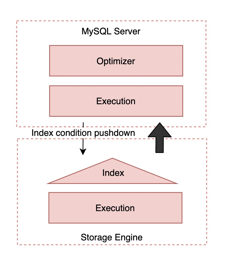
This stage is mainly used to directly display the summary information (including index) of each table in the execution plan condition pushdown information).
{
  "refine_plan": [
    {
      "table": "`t3`",
      "pushed_index_condition": "(`t3`.`name` = 'acb')",
      "table_condition_attached": null
    }
  ]
}
join_execution
This stage mainly displays the following information during implementation:
- Temporary table information
Here is the basic information of the temporary table in the execution plan. The important information includes location: disk (InnoDB),
{
  "creating_tmp_table": {
    "tmp_table_info": {
    "table": "intermediate_tmp_table",
    "in_plan_at_position": 8,
    "columns": 3,
    "row_length": 47,
    "key_length": 5,
    "unique_constraint": false,
    "makes_grouped_rows": true,
    "cannot_insert_duplicates": false,
    "location": "TempTable"
    }
  }
},- Sorting information
This contains the basic information of sorting, filesort_information; Whether to use optimized filesort for priority queue heap sorting_ priority_ queue_ Optimization, which is usually used by LIMIT; Memory and size used for sorting filesort_summary
{
  "sorting_table_in_plan_at_position": 8,
  "filesort_information": [
    {
      "direction": "asc",
      "table": "intermediate_tmp_table",
      "field": "o_year"
    }
  ],
  "filesort_priority_queue_optimization": {
    "usable": false,
    "cause": "not applicable (no LIMIT)"
  },
  "filesort_execution": [],
  "filesort_summary": {
    "memory_available": 262144,
    "key_size": 13,
    "row_size": 13,
    "max_rows_per_buffer": 15,
    "num_rows_estimate": 15,
    "num_rows_found": 2,
    "num_initial_chunks_spilled_to_disk": 0,
    "peak_memory_used": 32784,
    "sort_algorithm": "std::sort",
    "unpacked_addon_fields": "using_heap_table",
    "sort_mode": "<fixed_sort_key, rowid>"
  }
}
summary
This article focuses on Optimizer For the detailed content of trace, only by deeply understanding the content of the tool itself can we really analyze what the Optimizer has done, which indexes, costs and optimization methods have been selected, and why. Although the JSON result looks complex, it can still help DBA s find performance problems and verify some optimization methods. I hope this article will be helpful to you.