1 feasible set of portfolio

The weight variable in the portfolio can realize the mapping relationship between the expected return and return volatility of the portfolio. In portfolio theory, all possible portfolios are called feasible sets, and the effective frontier is an envelope of feasible sets. It represents the highest expected rate of return that can be brought to investors under different risk conditions, or the lowest volatility that can be brought to investors under different expected rates of return.

Next, take the portfolio composed of five stocks as an example to draw the feasible set of the portfolio. The Python program is as follows:

import numpy as np
import pandas as pd
import matplotlib.pyplot as plt 

plt.rcParams['font.sans-serif'] = ['SimHei'] #Chinese display problem
plt.rcParams['axes.unicode_minus'] = False #Negative numbers show problems


# Efficient frontier of portfolio
Rp_list = []
Vp_list = []
#Set the weight of each product in the portfolio
R_mean = np.array([0.20,0.08,-0.17,0.06,-0.04])
#Set the covariance of the portfolio
R_cov = pd.DataFrame({'A':[0.09,0.02,0.02,0.01,0.02],\
              'B':[0.02,0.12,0.04,0.02,0.03],\
              'C':[0.02,0.04,0.07,0.02,0.03],\
              'D':[0.01,0.02,0.02,0.04,0.02],\
              'E':[0.02,0.03,0.03,0.02,0.04]})
        

for i in np.arange(1000):
    #Randomly generate 1000 portfolio weights
    x = np.random.random(5)
    weights = x/sum(x)
    Rp_list.append(np.sum(weights*R_mean))
    Vp_list.append(np.sqrt(np.dot(weights,np.dot(R_cov,weights.T))))
    
   
plt.figure(figsize=(8,6))
plt.scatter(Vp_list,Rp_list)
plt.xlim(0.12,0.28)
plt.ylim(-0.1,0.2)
plt.xlabel('Volatility')
plt.ylabel('Expected rate of return')
plt.grid('True')

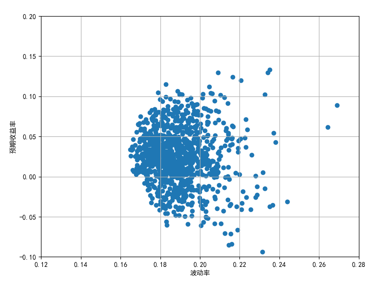
It can be seen from the feasible set that when the volatility is certain, rational investors will choose the top point of the feasible set to invest in order to maximize the rate of return; When the expected rate of return is certain, rational investors will choose the leftmost point of the feasible set to invest in order to minimize the return volatility (risk minimization).

2 efficient frontier of portfolio

Solving the effective frontier is to solve the following optimization problems:

m i n σ p = m i n ∑ ∑ w i w j C o v ( R i , R j ) about beam strip piece : ∑ w i = 1 w i > 0 E ( R p ) = ∑ w i E ( R i ) = C ( often number ) min\sigma_p = min\sqrt{\sum\sum w_iw_jCov(R_i,R_j)} \[10pt] constraints: \ \ [10pt] \ sum w_ i =1 \[10pt] w_ i > 0 \[10pt] E(R_p) = \sum w_ IE (r_i) = C (constant) minσp​=min∑∑wi​wj​Cov(Ri​,Rj​) Constraints: Σ wi = 1wi > 0e (RP) = Σ wi E(Ri) = C (constant)

w i > 0 w_i>0 wi > 0 as one of the constraints indicates that short selling of stocks is not allowed (i.e. short selling is not allowed in China).

When solving the above optimization problems, you need to use the minimize function in the Scipy sub module optimize( Please refer to the official website for details ), its usage is as follows:

'''
scipy.optimize.minimize(fun, x0, args=(), method=None, jac=None, hess=None, hessp=None, bounds=None, constraints=(), tol=None, callback=None, options=None)
fun:Optimal objective function
x0: Initial guess value
method: Optimization methods, commonly used methods are'BFGS','SLSQP'etc.
bounds: Boundary value of variable, tuple form
constraints: Constraints, dictionary form({'type':'eq','fun':Constraint I},{'type':'ineq','fun':Constraint 2})，'eq'Means equal to 0,'ineq'Indicates greater than or equal to 0
 Return value
fun:Objective function value
sucess:Boolean, true success
x:Optimal solution
'''
# Solve the optimal weight
import scipy.optimize as sco

#Define an optimization function
def f(w):
    w = np.array(w) #Set the weight of each stock in the portfolio
    Rp_opt = np.sum(w*R_mean) #Calculate the expected rate of return of the optimal portfolio
    Vp_opt = np.sqrt(np.dot(w,np.dot(R_cov,w.T))) #Calculate the return volatility of the optimal portfolio
    return np.array([Rp_opt,Vp_opt])

def Vmin_f(w): 
    return f(w)[1]  #Returns the volatility of the result of the f(w) function

#Enter the optimal solution conditions and set the expected return at 10%
cons = ({'type':'eq','fun':lambda x:np.sum(x)-1},{'type':'eq','fun':lambda x:f(x)[0]-0.1})
#Input boundary conditions
bnds = tuple((0,1) for x in range(len(R_mean)))
#Generate initial weights (evenly distributed)
frist_weight = len(R_mean)*[1/len(R_mean)]

#Find the most value
result = sco.minimize(Vmin_f,frist_weight,method='SLSQP',bounds=bnds,constraints=cons)
# Get the weight of the optimization result
result['x'].round(4)
for i in np.arange(len(R_cov)):
    print('Expected return on portfolio 10%Time' + R_cov.columns[i] +'Weight of:',result['x'][i].round(4))

#When the expected return of the portfolio is 10%, the weight of A: 0.3109
#When the expected return of the portfolio is 10%, the weight of B is 0.0859
#When the expected return of the portfolio is 10%, the weight of C is 0.0
#Weight of D when the expected rate of return of the portfolio is 10%: 0.5507
#The weight of E when the expected rate of return of the portfolio is 10%: 0.0525

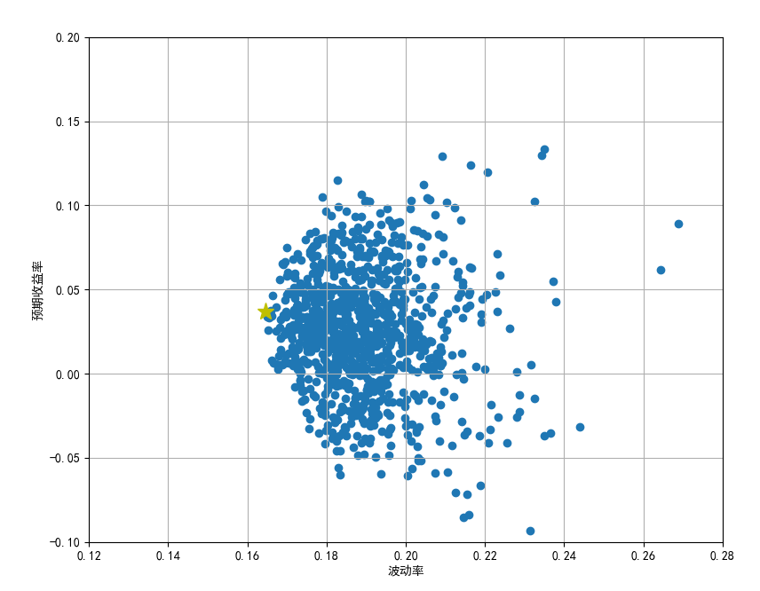
Next, the global minimum volatility of the portfolio and the corresponding expected rate of return are solved. The Python program is as follows:

#Solve the leftmost point of the effective leading edge
#The constraint only sets the sum of the weights to 1
cons_vmin = ({'type':'eq','fun':lambda x:np.sum(x)-1})
#Weight of global optimal solution
result_vmin = sco.minimize(Vmin_f,frist_weight,method='SLSQP',bounds=bnds,constraints=cons_vmin)
#Solve the yield of the leftmost point of the portfolio
Rp_vmin = np.sum(R_mean*result_vmin['x'])
#Solve the volatility of the leftmost point of the portfolio
Vp_vmin = result_vmin['fun']

print('Yield of the leftmost point of the portfolio feasible set:',round(Rp_vmin,4))
print('Volatility of the leftmost point of the portfolio feasible set:',round(Vp_vmin,4))

#Yield at the leftmost point of portfolio feasible set: 0.0371
#Volatility of the leftmost point of the portfolio feasible set: 0.1645

plt.plot(Vp_vmin,Rp_vmin,'y*',markersize=14)

Given the expected rate of return of a group of portfolios, the above function can be used to solve the corresponding minimum volatility, that is, the minimum volatility corresponding to the expected rate of return. These expected rates of return and their corresponding minimum volatility constitute the effective frontier. The Python program is as follows:

#Solve the curve formed by the effective front
#Set the expected rate of return of the portfolio
Rp_target = np.linspace(Rp_vmin,0.25,100)
#Set volatility list
Vp_target = []
for r in Rp_target:
    cons_new = ({'type':'eq','fun':lambda x:np.sum(x)-1},{'type':'eq','fun':lambda x:f(x)[0]-r})
    result_new = sco.minimize(Vmin_f,frist_weight,method='SLSQP',bounds=bnds,constraints=cons_new)
    Vp_target.append(result_new['fun'])
    
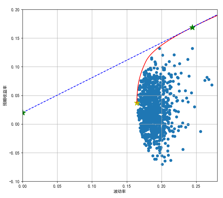
plt.plot(Vp_target,Rp_target,'r-')

3 capital market line

The assets used in the construction of the above portfolio are military risky assets and do not involve risk-free assets. If risk-free assets are included in the portfolio, investors can borrow or lend any amount of funds at the risk-free interest rate, which leads to the capital market line.

The capital market line is a tangent line derived from the risk-free rate of return and tangent to the effective frontier. There is one and only one, and its expression is as follows:

E ( R P ) = R f + E ( R M ) − R f σ M σ P E(R_P) = R_f + \frac{E(R_M)-R_f}{\sigma_M}\sigma_P E(RP​)=Rf​+σM​E(RM​)−Rf​​σP​

Among them, R f R_f Rf = risk-free rate of return, E ( R M ) E(R_M) E(RM) and σ M \sigma_M σ M ， respectively represents the market expected rate of return and volatility, represented by Portfolio performance evaluation It can be seen that the slope of the capital market line is the sharp ratio of the market portfolio.

The purpose of building a portfolio is to maximize benefits, that is, to solve the maximum slope of the capital market line is to solve the maximum value of the following formula:

m i n E ( R P ) − R f σ P about beam strip piece : ∑ w i = 1 w i > 0 min \frac{E(R_P)-R_f}{\sigma_P} \[10pt] constraints: \ \ [10pt] \ sum w_ i =1 \[10pt] w_ i > 0 min σ P − E(RP) − Rf constraints: Σ wi = 1wi > 0

Assuming that the risk-free rate of return is 2%, the procedure is as follows:

#CML (capital market line): consider the impact of risk-free assets
def F(w):
    Rf = 0.02
    w = np.array(w)
    Rp_opt = np.sum(w*R_mean)
    Vp_opt = np.sqrt(np.dot(w,np.dot(R_cov,w.T)))
    SR = (Rp_opt-Rf)/Vp_opt #Define the sharp ratio of the portfolio
    return np.array([Rp_opt,Vp_opt,SR])

def SRmin_F(w):
    return -F(w)[2] #Solving the maximum sharp ratio is solving the negative minimum

#Only set constraints where the sum of weights is 1
cons_SR = ({'type':'eq','fun':lambda x:np.sum(x)-1})
#Solve the optimal weight
result_SR = sco.minimize(SRmin_F,frist_weight,method='SLSQP',bounds=bnds,constraints=cons_SR)

Rf= 0.02 #Risk free interest rate
#Maximum sharp ratio, i.e. slope of capital market line
slope = -result_SR['fun']
#Expected rate of return of market portfolio
Rm = np.sum(R_mean*result_SR['x'])
#Volatility of market portfolio
Vm = (Rm-Rf)/slope

print('Yield of market portfolio:',round(Rm,4))
print('Volatility of market portfolio:',round(Vm,4))

#Yield of market portfolio: 0.1688
#Volatility of market portfolio: 0.2442

#Draw the capital market line
Rp_cml = np.linspace(0.02,0.25)
Vp_cml = (Rp_cml - Rf)/slope
plt.plot(Vp_cml,Rp_cml,'b--')
plt.plot(Vm,Rm,'g*',markersize=14)