This forecast relates to the marketing activities of Portuguese banking institutions. These marketing activities are generally based on telephone. The customer service personnel of the bank contact the customer at least once to confirm whether the customer is willing to buy the bank's products (time deposit). The basic type of task is classified task, which is to predict whether the customer will buy the bank's products.
Related package
import pandas as pd
import numpy as np
import matplotlib.pyplot as plt
import seaborn as sns
import warnings
warnings.filterwarnings("ignore")
from sklearn import ensemble,
from sklearn import model_selection
from sklearn import multiclass
from sklearn.model_selection import cross_val_score
from sklearn.preprocessing import OneHotEncoder, LabelEncoder
from sklearn.metrics import roc_curve, auc,roc_auc_score
from sklearn.metrics import classification_report, confusion_matrix
from sklearn.metrics import confusion_matrix
from sklearn.metrics import ConfusionMatrixDisplay
from sklearn.model_selection import GridSearchCV
from imblearn.over_sampling import SMOTE
from scipy.stats import chi2_contingency
Data preprocessing
Data import
train_set = pd.read_csv('train_set.csv')
test_set = pd.read_csv('test_set.csv')
print(train_set.shape)
print(test_set.shape)
#(25317, 18)
#(10852, 17)
#train_set.info()
#test_set.info()
Data field
ID: customer unique ID
Age: age
job: position
Marital: marital status
education: education
Default: whether there is a default record
Balance: the average balance of the account every year
Housing: is there a housing loan
Loan: is there a personal loan
contact: communication with customers
Last contact date: day
Month: the month of the last contact
Duration: the communication duration of the last contact
campaign: the number of exchanges with customers in this activity
pdays: how long has it been since the last time the customer was contacted in the last activity (999 means no contact)
previous: the number of times we communicated with the customer before this activity
poutcome: the result of the last activity
y: Predict whether customers will order time deposit business
Duplicate value processing
test_set = test_set.drop_duplicates()
train_set = train_set.drop_duplicates()
print(train_set.shape)
print(test_set.shape)
#(25317, 18)
#(10852, 17)
#The data has no duplicate values
Missing value processing
#The data has no NA value but has an unknow n value
train_set.isin(['unknown']).mean()*100
#job:0.643836,education:4.206660,contact:28.759332,poutcome:81.672394
test_set.isin(['unknown']).mean()*100
#job:0.552893,education:4.128271,contact:28.676742,poutcome:81.800590
# Work, education and communication methods are filled with modes. The result of the last communication is poutcome. This feature is abandoned because there are too many deficiencies
train_set.drop(['poutcome'],inplace=True,axis=1)
train_set['job'].replace(['unknown'],train_set['job'].mode(),inplace=True)
train_set['education'].replace(['unknown'],train_set['education'].mode(),inplace=True)
train_set['contact'].replace(['unknown'],train_set['contact'].mode(),inplace=True)
test_set.drop(['poutcome'],inplace=True,axis=1)
test_set['job'].replace(['unknown'],test_set['job'].mode(),inplace=True)
test_set['education'].replace(['unknown'],test_set['education'].mode(),inplace=True)
test_set['contact'].replace(['unknown'],test_set['contact'].mode(),inplace=True)
Exploratory analysis
#Discrete variable column name
object_columns = ['job', 'marital', 'education', 'default', 'housing', 'loan', 'contact','month']
#Continuous variable column name
num_columns = ['age', 'balance', 'duration', 'campaign', 'pdays', 'previous','day']
discrete variable
def barplot(x,y, **kwargs):
    sns.barplot(x=x , y=y)
    x = plt.xticks(rotation=45)
f = pd.melt(train_set,  value_vars=object_columns ,id_vars = 'y')
g = sns.FacetGrid(f, col="variable", col_wrap=3, sharex=False, sharey=False, size=5)
g = g.map(barplot,"value",'y')
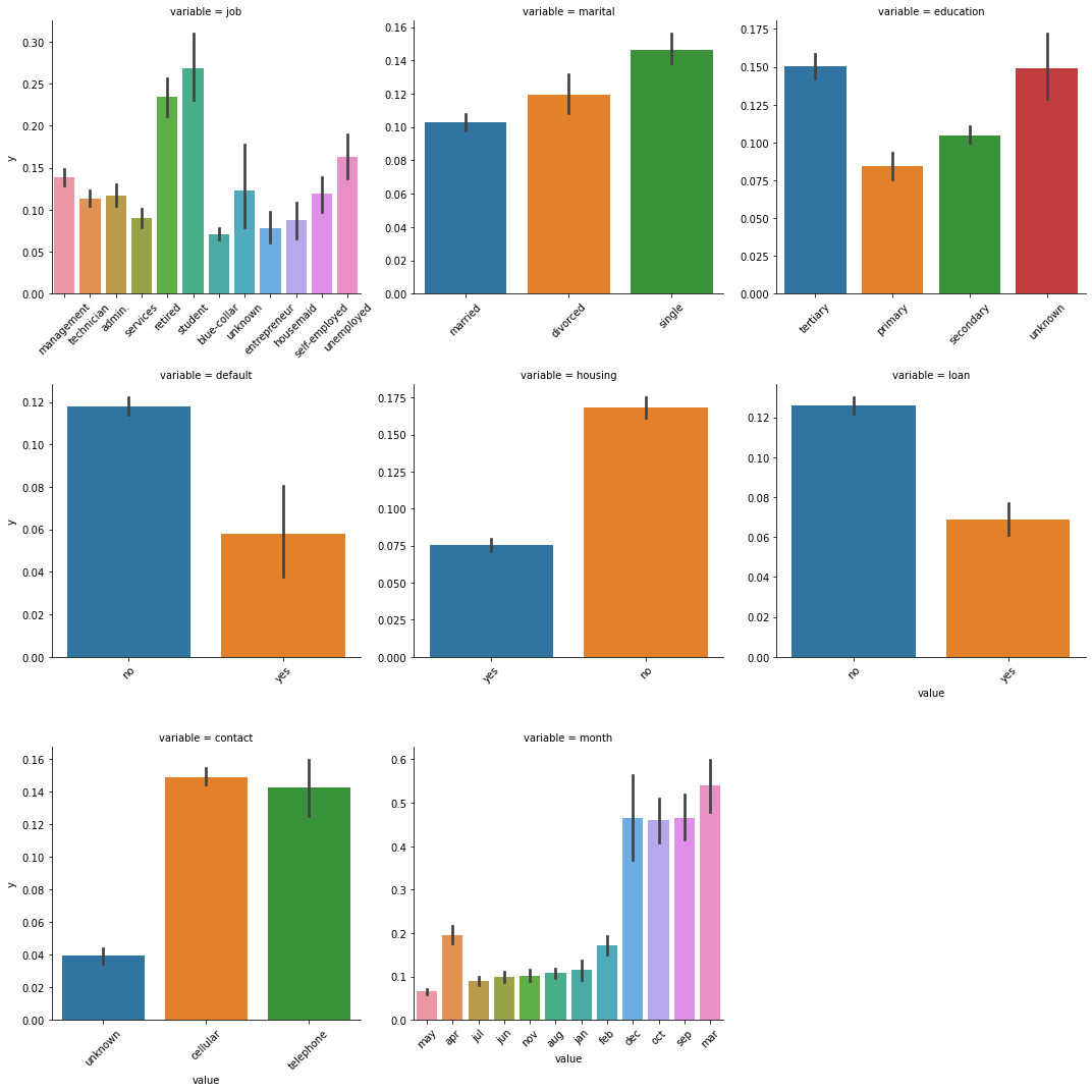
Position: retirees and students are more likely to buy time deposits, followed by the unemployed and managers, and the willingness of blue collar fixed-term financial management is lower
Marital status: single people are more willing to manage money regularly than divorced and married people
Education level: the willingness of regular financial management is reduced according to the education level of University, high school and junior middle school
Whether there is a default record: people without a default record are twice as likely to buy regular financial management as those with a default record
Whether there is housing loan: people without housing loan may buy fixed-term financial management more than twice as much as those with housing loan
Whether there is personal loan: people without personal loan are more likely to buy fixed-term financial management
Communication with customers: communication by telephone and mobile phone has no obvious impact on customers' decision to purchase time deposits
The last contact month: December, October, September and March, the proportion of time deposits purchased is high
g = sns.FacetGrid(train_set, col='marital',size=5)
g.map(sns.barplot, 'default', 'y', 'education')
g.add_legend()
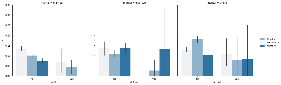
Single people with no record of default and college degree are more likely to buy time deposits
People with divorce, a record of default and a college degree are less likely to buy time deposits
def barplot(x,y, **kwargs):
    sns.barplot(x=x , y=y)
    x=plt.xticks(rotation=90)

plt.figure(figsize=(16, 12))
g = sns.FacetGrid(train_set, col='education',col_order=['primary','secondary','tertiary'],size=5)
g.map(barplot, 'job', 'y')
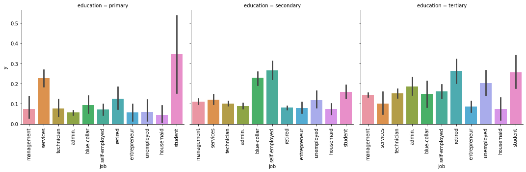
With the improvement of educational background, the willingness of retirees and blue collar workers to buy regular financial management increases, while the willingness of students to buy regular financial management decreases
continuous variable
f = pd.melt(train_set,  value_vars=num_columns ,id_vars = 'y')
g = sns.FacetGrid(f, col="variable", col_wrap=3, sharex=False, sharey=False, size=5,hue='y')
g = g.map(sns.distplot,"value",bins=20)
g.add_legend()
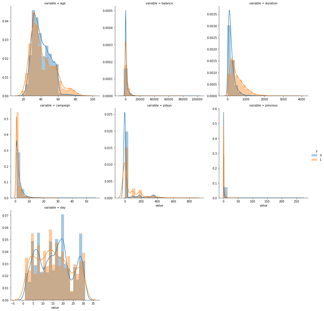
Age: more willing to buy regular financial products before the age of 30, less willing to buy regular financial products at the age of 30-60, and significantly more likely to buy regular financial products after the age of 60
Communication duration: the rate of purchasing fixed-term financial management increased after about 300 minutes of communication
Number of communication with customers in this activity: the increase of communication times can not significantly improve the ratio of customers to buy regular financial management
How long has it been since the last time the customer was contacted in the last activity: in 140-160180-200 days, the rate of customers purchasing regular financial management has increased significantly
Number of communication with the customer before this activity: the increase of communication times can not significantly improve the ratio of customers to buy regular financial management, which may be counterproductive
Date: there will be three peak purchases of regular financial management every month, and customers least want to buy regular financial management on the 23rd-25th of each month
Characteristic Engineering
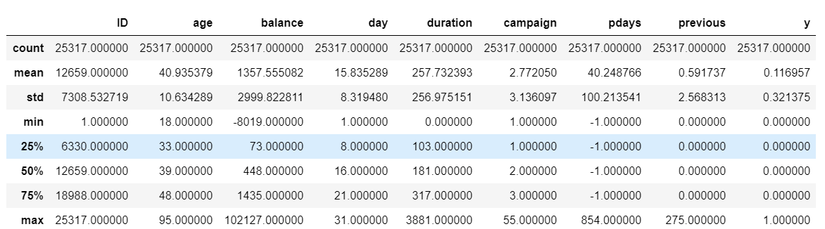
descriptive statistics
sns.countplot(train_set['y'])
#If the data distribution is unbalanced, up sampling can be used to solve the problem of sample imbalance

#descriptive statistics
train_set.describe()
test_set.describe()
#Distribution of data
categorical_features = ['balance','duration','campaign','pdays','previous']
f = pd.melt(train_set,  value_vars=categorical_features,id_vars=['y'])
g = sns.FacetGrid(f, col="variable",  col_wrap=3, sharex=False, sharey=False, size=5)
g = g.map(sns.boxplot, "value")

It can be seen that there are many extreme values of data. Deleting extreme values will have a certain impact on the source data. The data will be processed in boxes later
Characteristic structure
#View the values of category variables
for column in object_columns:
    print(column,':  ',train_set[column].unique())
#job :   ['management' 'technician' 'admin.' 'services' 'retired' 'student' 'blue-collar' 'entrepreneur' 'housemaid' 'self-employed' 'unemployed']
#marital :   ['married' 'divorced' 'single']
#education :   ['tertiary' 'primary' 'secondary']
#default :   ['no' 'yes']
#housing :   ['yes' 'no']
#loan :   ['no' 'yes']
#contact :   ['cellular' 'telephone']
#month :   ['may' 'apr' 'jul' 'jun' 'nov' 'aug' 'jan' 'feb' 'dec' 'oct' 'sep' 'mar']

#Characteristics of structural quarter and half year
def quarter(data):
    a = ''
    if data in ['jan','feb','mar']:
        a = 'Q1'
    elif data in ['apr','may','jun']:
        a = 'Q2'
    elif data in ['jul','aug','sep']:
        a = 'Q3'
    else:
        a = 'Q4'
    return a

def halfyear(data):
    a = ''
    if data in ['jan','feb','mar','apr','may','jun']:
        a = 'H1'
    else:
        a = 'H2'
    return a
The discrete data is encoded and the continuous data is divided into boxes. The methods of box division include equivalence, equal width, clustering, chi square, minimum entropy, etc. Here, qcut and cut are selectively used to divide the data according to the characteristics of the data, and the number of boxes is determined by woe and iv values.
def CalcWOE(df, col, target):
    '''
    : df dataframe
    : col Note that this column has been divided into boxes. Now calculate the weight of each box WOE And overall IV
    : target Target column 0-1 value
    : return Return each box WOE And overall IV
    '''
    total = df.groupby([col])[target].count()
    total = pd.DataFrame({'total': total})
    bad = df.groupby([col])[target].count() - df.groupby([col])[target].sum()
    bad = pd.DataFrame({'bad': bad})
    regroup = total.merge(bad, left_index=True, right_index=True, how='left')
    regroup.reset_index(level=0, inplace=True)
    N = sum(regroup['total'])
    B = sum(regroup['bad'])
    regroup['good'] = regroup['total'] - regroup['bad']
    G = N - B
    regroup['bad_pcnt'] = regroup['bad'].map(lambda x: x * 1.0 / B)
    regroup['good_pcnt'] = regroup['good'].map(lambda x: x * 1.0 / G)
    regroup['WOE'] = regroup.apply(
        lambda x: np.log(x.good_pcnt * 1.0 / x.bad_pcnt), axis=1)
    WOE_dict = regroup[[col, 'WOE']].set_index(col).to_dict(orient='index')
    IV = regroup.apply(
        lambda x:
        (x.good_pcnt - x.bad_pcnt) * np.log(x.good_pcnt * 1.0 / x.bad_pcnt),
        axis=1)
    IV_SUM = sum(IV)
    return {'WOE': WOE_dict, 'IV_sum': IV_SUM, 'IV': IV}

#Judge whether woe satisfies monotonicity
def BadRateMonotone(df, sortByVar, target):
    #df[sortByVar] this column has been divided into boxes
    df2 = df.sort_values(by=[sortByVar])
    total = df2.groupby([sortByVar])[target].count()
    total = pd.DataFrame({'total': total})
    bad = df2.groupby([sortByVar])[target].count() - df2.groupby(
        [sortByVar])[target].sum()
    bad = pd.DataFrame({'bad': bad})
    regroup = total.merge(bad, left_index=True, right_index=True, how='left')
    regroup.reset_index(level=0, inplace=True)
    combined = zip(regroup['total'], regroup['bad'])
    badRate = [x[1] * 1.0 / x[0] for x in combined]
    badRateMonotone = [
        badRate[i] < badRate[i + 1] for i in range(len(badRate) - 1)
    ]
    Monotone = len(set(badRateMonotone))
    if Monotone == 1:
        return True
    else:
        return False


def num_band(df, columns, target, min_num, max_num):
    result = []
    for col in columns:
        for i in range(min_num, max_num):
            try:
                df['band'] = pd.cut(df[col], i)
                WOE_IV = CalcWOE(df, 'band', target)
                T_F = BadRateMonotone(df, 'band', target)
                result.append([col, i, WOE_IV['IV_sum'], T_F])
            except:
                continue
    return pd.DataFrame(result, columns=['column', 'num', 'IV_sum', 'T_F'])


num_band(train_set, num_columns, 'y', 2, 10)
#Select woe the number of bins with monotonicity and maximum IV value
for dataset in [train_set]:
    dataset['balanceBin'] = pd.qcut(dataset['balance'], 5)
    dataset['ageBin'] = pd.cut(dataset['age'].astype(int), [0, 30, 60, 100])
    dataset['quarter'] = dataset['month'].map(quarter)
    dataset['halfyear'] = dataset['month'].map(halfyear)
    dataset['dayBin'] = pd.cut(dataset['day'], 2)
    dataset['durationBin'] = pd.qcut(dataset['duration'], 9)
    dataset['campaignBin'] = pd.qcut(dataset['campaign'], 2)
    dataset['pdaysBin'] = pd.cut(dataset['pdays'], 9)
    dataset['previousBin'] = pd.cut(dataset['previous'], 9)
    dataset['all_previous'] = dataset['campaign'] + dataset['previous']
    dataset['all_previousBin'] = pd.cut(dataset['all_previous'], 2)
Feature screening
Judge the maximum proportion of each category (box division result) in the overall proportion. If the proportion of a category exceeds 95%, it indicates that this feature is seriously skewed, and the feature should be removed. The final result is to remove previousBin and all_previousBin feature
def MaximumBinPcnt(df, col):
    N = df.shape[0]
    total = df.groupby([col])[col].count()
    pcnt = total * 1.0 / N
    return max(pcnt)

discrete_columns = [
    'job', 'marital', 'education', 'default', 'housing', 'loan', 'contact',
    'month', 'y', 'balanceBin', 'ageBin', 'quarter', 'halfyear', 'dayBin',
    'durationBin', 'campaignBin', 'pdaysBin', 'previousBin', 'all_previousBin'
]

for column in discrete_columns:
    print(column, ':', MaximumBinPcnt(train_set, column))
Encode data labels
label = LabelEncoder()
for dataset in [train_set]:
    dataset['job_Code'] = label.fit_transform(dataset['job'])
    dataset['ageBin_Code'] = label.fit_transform(dataset['ageBin'])
    dataset['marital_Code'] = label.fit_transform(dataset['marital'])
    dataset['education_Code'] = label.fit_transform(dataset['education'])
    dataset['default_Code'] = label.fit_transform(dataset['default'])
    dataset['balanceBin_Code'] = label.fit_transform(dataset['balanceBin'])
    dataset['housing_Code'] = label.fit_transform(dataset['housing'])
    dataset['loan_Code'] = label.fit_transform(dataset['loan'])
    dataset['contact_Code'] = label.fit_transform(dataset['contact'])
    dataset['dayBin_Code'] = label.fit_transform(dataset['dayBin'])
    dataset['month_Code'] = label.fit_transform(dataset['month'])
    dataset['durationBin_Code'] = label.fit_transform(dataset['durationBin'])
    dataset['campaignBin_Code'] = label.fit_transform(dataset['campaignBin'])
    dataset['pdaysBin_Code'] = label.fit_transform(dataset['pdaysBin'])
    dataset['quarter_Code'] = label.fit_transform(dataset['quarter'])
    dataset['halfyear_Code'] = label.fit_transform(dataset['halfyear'])
Use chi square test to screen discrete variables,
for col in columns_train_data_x:
    obs = pd.crosstab(train_set['y'],
                      train_set[col],
                      rownames=['y'],
                      colnames=[col])
    chi2, p, dof, expect = chi2_contingency(obs)
    print("{} Chi square test p value: {:.4f}".format(col, p))
#The P value of chi square test for all features was significantly less than 0.01, and all features were retained

columns_train_data_x = [
    'job_Code', 'ageBin_Code', 'marital_Code', 'education_Code',
    'default_Code', 'balanceBin_Code', 'housing_Code', 'loan_Code',
    'contact_Code', 'dayBin_Code', 'month_Code', 'durationBin_Code',
    'campaignBin_Code', 'pdaysBin_Code', 'quarter_Code', 'halfyear_Code'
]
Target = ['y']
#spearman is used to test the correlation between the data
def correlation_heatmap(df):
    _ , ax = plt.subplots(figsize =(20, 16))
    colormap = sns.diverging_palette(220, 10, as_cmap = True)

    _ = sns.heatmap(
        df.corr('spearman'),
        cmap = colormap,
        square=True,
        cbar_kws={'shrink':.9 },
        ax=ax,
        annot=True,
        linewidths=0.1,vmax=1.0, linecolor='white',
        annot_kws={'fontsize':10 }
    )

    plt.title('Pearson Correlation of Features', y=1.05, size=15)

correlation_heatmap(train_set[columns_train_data_xy])
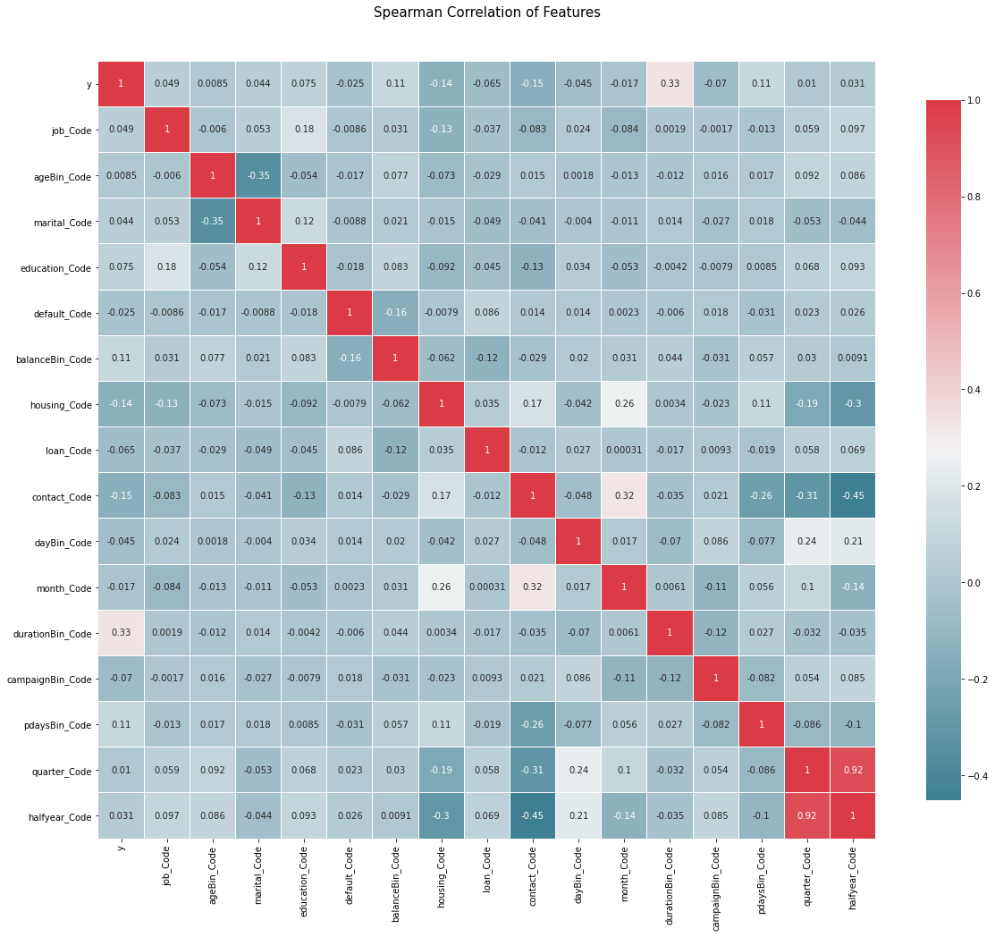 quarter_Code and halfyear_Code is highly relevant, so only halfyear is selected_ Code
Modeling analysis
Training data
columns_train_data_x = [
    'job_Code', 'ageBin_Code', 'marital_Code', 'education_Code',
    'default_Code', 'balanceBin_Code', 'housing_Code', 'loan_Code',
    'contact_Code', 'dayBin_Code', 'month_Code', 'durationBin_Code',
    'campaignBin_Code', 'pdaysBin_Code', 'halfyear_Code'
]
train_data_x = train_set[columns_train_data_x]
train_data_y = train_set['y']
train_data_x = pd.get_dummies(train_data_x , columns=columns_train_data_x)
The samples are up sampled by BorderlineSMOTE, ADASYN, SMOTETomek, etc
#Oversampling samples
train_data_x,train_data_y = SMOTE().fit_resample(train_data_x,train_data_y)
train_data_y.value_counts()
#0    22356
#1    22356
GBDT
The full name of GBDT is Gradient Boosting Decision Tree, which is an integrated learning algorithm and is widely used in industry.
The grid search and optimization of GBDT can be carried out directly. If the amount of data is too large, the greedy algorithm can be used for optimization, but the greedy algorithm can only achieve local optimization.
GBDT_n_estimators = [120, 300]
GBDT_learning_rate = [0.001, 0.01]
GBDT_max_features = ['sqrt']
GBDT_max_depth = [3, 5, 8]
#GBDT_min_samples_split = [1, 2, 5, 10, 15, 100]
#GBDT_min_samples_leaf = [1, 2, 5, 10]
#GBDT_subsample = [0.5, 0.6, 0.7, 0.8, 0.9, 1]

param_grid = {
    'n_estimators': GBDT_n_estimators,
    'learning_rate': GBDT_learning_rate,
    'max_features': GBDT_max_features,
    'max_depth': GBDT_max_depth,
    #'min_samples_split': GBDT_min_samples_split,
    #'min_samples_leaf': GBDT_min_samples_leaf,
    #'subsample': GBDT_subsample
}
cv_split = model_selection.ShuffleSplit(n_splits=10,
                                        test_size=.3,
                                        random_state=0)
model_tunning = GridSearchCV(ensemble.GradientBoostingClassifier(),
                             param_grid=param_grid,
                             cv=cv_split,
                             scoring='roc_auc')
model_tunning.fit(train_data_x, train_data_y)
print('Optimal score', model_tunning.best_score_)  #Model maximum score
print('Optimal parameters', model_tunning.best_params_)  #Optimal parameters
print('Optimal model', model_tunning.best_estimator_)  #Optimal model
best_model = model_tunning.best_estimator_
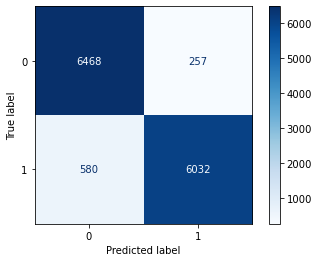
Model evaluation methods include confusion matrix, accuracy rate, recall rate, ROC curve, ACU value, etc
#Confusion matrix
x_train, x_test, y_train, y_test = model_selection.train_test_split(
    train_data_x, train_data_y, train_size=.7)
model = ensemble.GradientBoostingClassifier(n_estimators=300,
                                            learning_rate=0.1,
                                            max_features='sqrt',
                                            max_depth=7,
                                            min_samples_split=500,
                                            min_samples_leaf=60,
                                            subsample=1)
model.fit(x_train, y_train)
y_predict = model.predict(x_test)
cm = confusion_matrix(y_test, y_predict)
ConfusionMatrixDisplay(cm).plot(cmap='Blues')
from sklearn.metrics import accuracy_score, precision_score,recall_score
print(accuracy_score(y_test, y_predict))  #Accuracy
print(precision_score(y_test, y_predict, average='weighted'))  #Weighted accuracy
print(recall_score(y_test, y_predict))  #recall
K-fold cross validation, ROC was used as the evaluation method_ auc
score = cross_val_score(model, train_data_x, train_data_y, cv=5, n_jobs=1, scoring='roc_auc')
score.mean()
#Final model score 0.9830339716115262
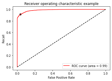
ROC curve
#ROC/AUC
model.fit(x_train, y_train)
def get_rocauc(y,X,clf):
    FPR,recall,thresholds=roc_curve(y,clf.predict_proba(X)[:,1],pos_label=1)
    area=roc_auc_score(y,clf.predict_proba(X)[:,1])

    maxindex=(recall-FPR).tolist().index(max(recall-FPR))
    threshold=thresholds[maxindex]

    plt.figure()
    plt.plot(FPR,recall,color='red',label='ROC curve (area = %0.2f)'%area)
    plt.plot([0,1],[0,1],color='black',linestyle='--')
    plt.scatter(FPR[maxindex],recall[maxindex],c='black',s=30)
    plt.xlim([-0.05,1.05])
    plt.ylim([-0.05,1.05])
    plt.xlabel('False Positive Rate')
    plt.ylabel('Recall')
    plt.title('Receiver operating characteristic example')
    plt.legend(loc='lower right')
    plt.show()
    return threshold

threshold=get_rocauc(y_test, x_test,model)
You are welcome to communicate and criticize