In the previous two talks, only risky assets are considered in portfolio allocation, but actually, risk-free assets (such as treasury bonds) may also be included in investment. What are the characteristics of investment under this situation? This leads to another concept - capital market line.
The capital market line (CML) is a straight line derived from the risk-free rate of return and tangent to the effective frontier. The slope of the straight line is only related to the risk-free rate of return. Therefore, when the risk-free rate of return is determined, the straight line will be determined.
I saw two pictures on Zhihu, which explained the capital market line in great detail, so I borrowed them and talked about them roughly. The article address is:

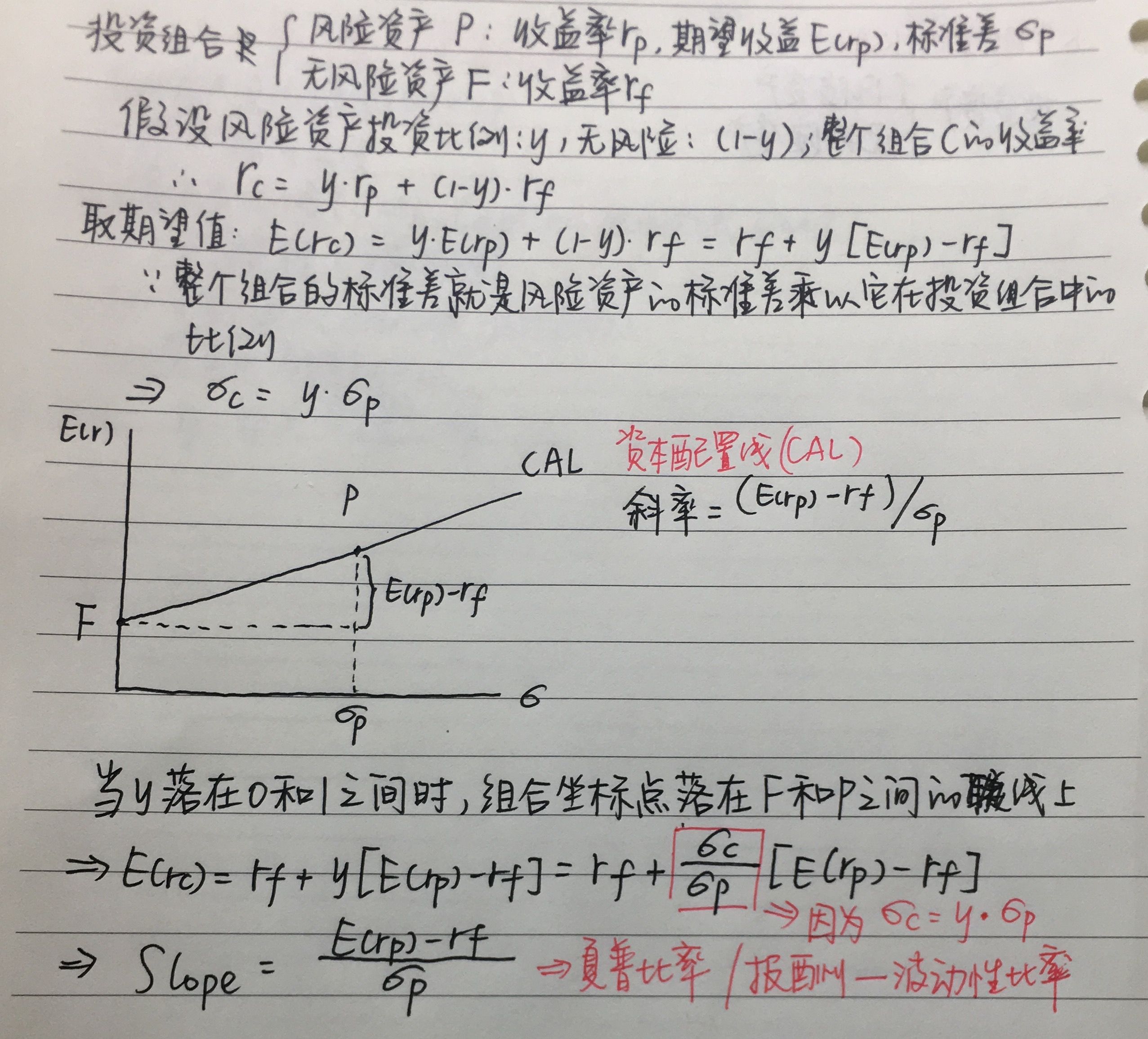
It can be seen from this figure that the capital allocation line is a ray derived from the risk-free return rate after the introduction of risk-free assets, and its slope is ( E ( R ) − R f ) / σ p (E(R)-Rf)/\sigma_p (E(R)−Rf)/ σ p, the ratio of the difference between the immediate expected return and the risk-free return to the volatility of the yield, which is also known as the sharp ratio.

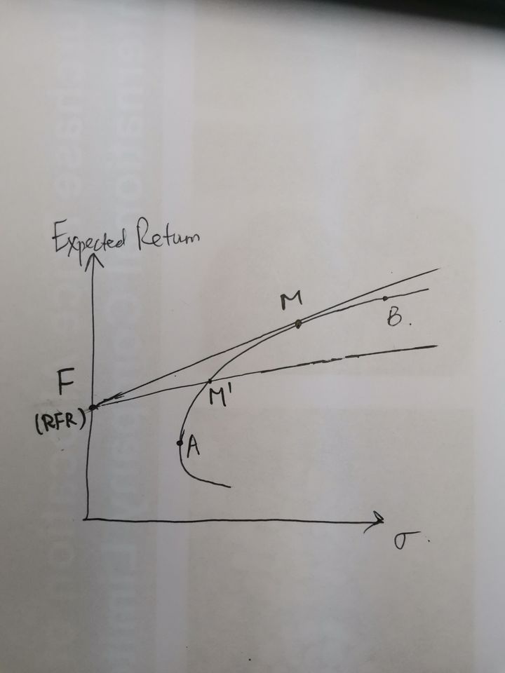
It can be seen from this figure that when the risk-free rate of return is determined, there can be many capital allocation lines, but only one can be tangent to the effective frontier, then this line is the capital market line, and the portfolio corresponding to the tangent point is called the market portfolio. Moreover, from these lines, we can also find that for the feasible set, when the risk (x) is the same, the capital market line can reach the maximum rate of return (y); When the returns are the same (y), the capital market line can obtain the minimum risk (x).
Therefore, the slope of the capital market line can actually be transformed into an equation with constraints to find the optimal solution:
Constraints are ∑ k = 1 n w i = 1 \displaystyle \sum_{k=1}^n w_i =1 k=1∑n​wi​=1， w i w_i wi > 0, the equation is
m a x   ( E ( R p ) − R f ) / σ p max\ (E(R_p)-R_f )/ \sigma_p max (E(Rp​)−Rf​)/σp​
Next, assuming that the risk-free interest rate is 3% / year, we still use the previous data to draw the capital market line. Let's do the whole process again:

#The purpose of obtaining the basic information table of stocks is to get the codes of the first few stocks
import tushare as ts
pro=ts.pro_api('b497571a3ddd7dde8ebe28b372879594b2f8356c918ad80dae01605b')
df=pro.stock_basic(exchange='', list_status='L', fields='ts_code,symbol,name,area,industry,list_date')
df.head()    

Then obtain the data and calculate the yield after processing:

import pandas as pd
dt=pd.DataFrame()
for i in df.loc[:5][['ts_code','name']].values:
    dt[i[1]]=pro.daily(ts_code=i[0], start_date='20180101', end_date='20210731')['close']
dt.drop('Guohua Wangan',axis=1,inplace=True)
import numpy as np
r=np.log(dt/dt.shift(1))
r=r.dropna()
r

Then calculate the relevant annualized return, covariance coefficient, correlation coefficient and volatility

r_mean=r.mean()*252
r_cov=r.cov()*252
r_corr=r.corr()
r_vol=r.std()*np.sqrt(252)
r_mean,r_cov,r_corr,r_vol

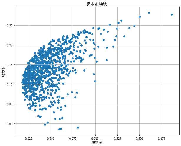
Draw the feasible set of the portfolio:

from pylab import mpl
mpl.rcParams['font.sans-serif']=['SimHei']
mpl.rcParams['axes.unicode_minus']=False
rp=[]
vp=[]
for i in np.arange(1000):
    x=np.random.random(5)
    weights=x/sum(x)
    rp.append(np.sum(weights*r_mean))
    vp.append(np.sqrt(np.dot(weights,np.dot(r_cov,weights.T))))
plt.figure(figsize=(10,8))
plt.scatter(vp,rp)
plt.xlabel(u'Volatility',fontsize=12)
plt.ylabel(u'Yield',fontsize=12,rotation=90)
plt.title(u'Capital market line',fontsize=14)
plt.grid('True')
plt.show()

Then calculate and draw the effective front:

import scipy.optimize as sco
def f(w):
    w=np.array(w)
    rp=np.sum(w*r_mean)
    vp=np.sqrt(np.dot(w,np.dot(r_cov,w.T)))
    return np.array([rp,vp])
def vmin(w):
    return f(w)[1]
cons=({'type':'eq','fun':lambda x:np.sum(x)-1})
bnds=tuple((0,1) for x in range(len(r_mean)))
result_min=sco.minimize(vmin,len(r_mean)*[1.0/len(r_mean),],method='SLSQP',bounds=bnds,constraints=cons)
rp_min=np.sum(r_mean*result_min['x'])
vp_min=result_min['fun']
rpt=np.linspace(rp_min,0.3,100)
vpt=[]
for i in rpt:
    cons=({'type':'eq','fun':lambda x:np.sum(x)-1},{'type':'eq','fun':lambda x:f(x)[0]-i})
    result=sco.minimize(vmin,len(r_mean)*[1.0/len(r_mean),],method='SLSQP',bounds=bnds,constraints=cons)
    vpt.append(result['fun'])
plt.figure(figsize=(10,8))
plt.scatter(vp,rp)
plt.plot(vpt,rpt,'r-',label=u'Effective frontier',lw=2)
plt.plot(vp_min,rp_min,'y*',label=u'Global minimum volatility',markersize=14)
plt.xlabel(u'Volatility',fontsize=12)
plt.ylabel(u'Yield',fontsize=12,rotation=90)
plt.title(u'Capital market line',fontsize=14)
plt.grid('True')
plt.show()

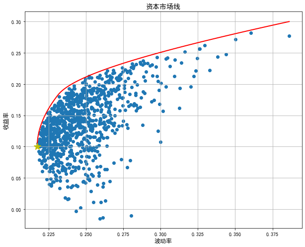
Then, assuming that the risk-free rate of return is 2%, calculate the slope of the capital market line and the market portfolio, and draw:

#Define correlation function
def ff(w):
    rf=0.02
    w=np.array(w)
    rp=np.sum(w*r_mean)
    vp=np.sqrt(np.dot(w,np.dot(r_cov,w.T)))
    sharp=(rp-rf)/vp
    return np.array([rp,vp,sharp])
def spmin(w):
    return -ff(w)[2]

#Calculate market mix
cons1=({'type':'eq','fun':lambda x:np.sum(x)-1})
result_s=sco.minimize(spmin,len(r_mean)*[1.0/len(r_mean),],method='SLSQP',bounds=bnds,constraints=cons1)
rf=0.02
slope=-result_s['fun']
rm=np.sum(r_mean*result_s['x'])
vm=(rm-rf)/slope
print(slope,rm,vm)

#Draw the entire drawing
rp_cml=np.linspace(0.02,0.3)
vp_cml=(rp_cml-rf)/slope
plt.figure(figsize=(10,8))
plt.scatter(vp,rp)
plt.plot(vpt,rpt,'r-',label=u'Effective frontier',lw=2)
plt.plot(vp_cml,rp_cml,'b--',label=u'Capital market line',lw=2)
plt.plot(vp_min,rp_min,'y*',label=u'Global minimum volatility',markersize=14)
plt.xlabel(u'Volatility',fontsize=12)
plt.ylabel(u'Yield',fontsize=12,rotation=90)
plt.title(u'Capital market line',fontsize=14)
plt.legend(fontsize=12)
plt.grid('True')
plt.show()

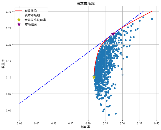
Finally, the graph of capital market line is obtained: