Five implementation strategies of pytoch's spatial shift operation
This article has authorized the platform of the polar city and is the official account of the polar platform. No second reprint is allowed without permission
Original document (may be further updated): https://www.yuque.com/lart/ug...
preface
Previously, I read some papers that use spatial offset operation to replace regional convolution operation:
Rough view: https://www.yuque.com/lart/ar...
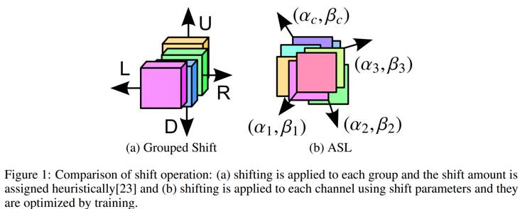
- (CVPR 2018) [Grouped Shift] Shift: A Zero FLOP, Zero Parameter Alternative to Spatial Convolutions:
- (ICCV 2019) 4-Connected Shift Residual Networks
- (NIPS 2018) [Active Shift] Constructing Fast Network through Deconstruction of Convolution
- (CVPR 2019) [Sparse Shift] All You Need Is a Few Shifts: Designing Efficient Convolutional Neural Networks for Image Classification
Take a closer look:
- Hire-MLP: Vision MLP via Hierarchical Rearrangement:https://www.yuque.com/lart/pa...
- CycleMLP: A MLP-like Architecture for Dense Prediction:https://www.yuque.com/lart/pa...
- S2-MLP: Spatial-Shift MLP Architecture for Vision:https://www.yuque.com/lart/pa...
- S2-MLPv2: Improved Spatial-Shift MLP Architecture for Vision:https://www.yuque.com/lart/pa...
After reading these papers, by referring to the core code provided by them (mainly the later MLP methods), I have some ideas on realizing spatial offset
By integrating the existing knowledge, I summarized five implementation strategies
Since I personally use pytorch, the presentation here may also use some useful functions provided by pytorch itself
Problem description
Before providing implementation, we should clarify the purpose in order to facilitate subsequent implementation
These existing works can be simplified as follows:
Given tensor $X \in \mathbb{R}^{1 \times 8 \times 5 \times 5} $, the default data format of pytorch is followed here, that is, B, C, H, W
Convert $x $to $\ tilde{X} $. By transforming $\ mathcal{T}: x \rightarrow \tilde{x} $
Here, tensor $\tilde{X} \in \mathbb{R}^{1 \times 8 \times 5 \times 5} $. In order to provide reasonable comparison, the results based on the "slice index" strategy in the following chapters are used as the value of $\ tilde{X} $
import torch

xs = torch.meshgrid(torch.arange(5), torch.arange(5))
x = torch.stack(xs, dim=0)
x = x.unsqueeze(0).repeat(1, 4, 1, 1).float()
print(x)

'''
tensor([[[[0., 0., 0., 0., 0.],
          [1., 1., 1., 1., 1.],
          [2., 2., 2., 2., 2.],
          [3., 3., 3., 3., 3.],
          [4., 4., 4., 4., 4.]],

         [[0., 1., 2., 3., 4.],
          [0., 1., 2., 3., 4.],
          [0., 1., 2., 3., 4.],
          [0., 1., 2., 3., 4.],
          [0., 1., 2., 3., 4.]],

         [[0., 0., 0., 0., 0.],
          [1., 1., 1., 1., 1.],
          [2., 2., 2., 2., 2.],
          [3., 3., 3., 3., 3.],
          [4., 4., 4., 4., 4.]],

         [[0., 1., 2., 3., 4.],
          [0., 1., 2., 3., 4.],
          [0., 1., 2., 3., 4.],
          [0., 1., 2., 3., 4.],
          [0., 1., 2., 3., 4.]]]])
'''
Method 1: slice index
This is the most direct and simple strategy This is also the strategy used in the S2-MLP series
We use it as a reference for all other strategies This result will also be obtained in subsequent implementations
direct_shift = torch.clone(x)
direct_shift[:, 0:2, :, 1:] = torch.clone(direct_shift[:, 0:2, :, :4])
direct_shift[:, 2:4, :, :4] = torch.clone(direct_shift[:, 2:4, :, 1:])
direct_shift[:, 4:6, 1:, :] = torch.clone(direct_shift[:, 4:6, :4, :])
direct_shift[:, 6:8, :4, :] = torch.clone(direct_shift[:, 6:8, 1:, :])
print(direct_shift)

'''
tensor([[[[0., 0., 0., 0., 0.],
          [1., 1., 1., 1., 1.],
          [2., 2., 2., 2., 2.],
          [3., 3., 3., 3., 3.],
          [4., 4., 4., 4., 4.]],

         [[0., 0., 1., 2., 3.],
          [0., 0., 1., 2., 3.],
          [0., 0., 1., 2., 3.],
          [0., 0., 1., 2., 3.],
          [0., 0., 1., 2., 3.]],

         [[0., 0., 0., 0., 0.],
          [1., 1., 1., 1., 1.],
          [2., 2., 2., 2., 2.],
          [3., 3., 3., 3., 3.],
          [4., 4., 4., 4., 4.]],

         [[1., 2., 3., 4., 4.],
          [1., 2., 3., 4., 4.],
          [1., 2., 3., 4., 4.],
          [1., 2., 3., 4., 4.],
          [1., 2., 3., 4., 4.]],

         [[0., 0., 0., 0., 0.],
          [0., 0., 0., 0., 0.],
          [1., 1., 1., 1., 1.],
          [2., 2., 2., 2., 2.],
          [3., 3., 3., 3., 3.]],

         [[0., 1., 2., 3., 4.],
          [0., 1., 2., 3., 4.],
          [0., 1., 2., 3., 4.],
          [0., 1., 2., 3., 4.],
          [0., 1., 2., 3., 4.]],

         [[1., 1., 1., 1., 1.],
          [2., 2., 2., 2., 2.],
          [3., 3., 3., 3., 3.],
          [4., 4., 4., 4., 4.],
          [4., 4., 4., 4., 4.]],

         [[0., 1., 2., 3., 4.],
          [0., 1., 2., 3., 4.],
          [0., 1., 2., 3., 4.],
          [0., 1., 2., 3., 4.],
          [0., 1., 2., 3., 4.]]]])
'''
Method 2: feature map offset - torch roll
pytorch provides a function to directly offset the feature map, namely torch roll . This operation has been used in recent transformer papers and mlp, such as SwinTransformer and mlp AS-MLP.
Here is the pseudocode provided in the AS-MLP paper:
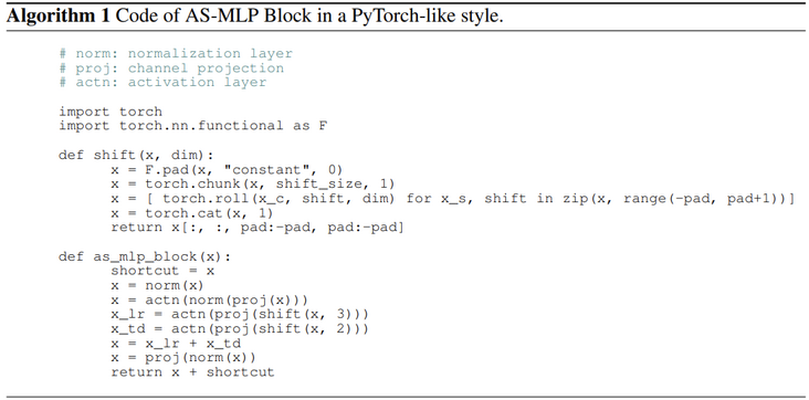
Its main function is to offset the feature map along a certain axis and support multiple axial offsets at the same time, so as to construct more diverse offset directions
In order to achieve the same result as before, we need to pad the input first
Because a characteristic of direct slice index is that boundary values will appear repeatedly, and direct roll operation will cause all values to move as a whole
Therefore, in order to achieve a similar effect, first pad a grid of data around
Note that repeat mode is selected here to achieve the effect of final boundary repeat value
import torch.nn.functional as F

pad_x = F.pad(x, pad=[1, 1, 1, 1], mode="replicate")  # Here, you need to use padding to preserve the boundary data
Next, start processing and offset the length by one unit in each of the four directions:
roll_shift = torch.cat(
    [
        torch.roll(pad_x[:, c * 2 : (c + 1) * 2, ...], shifts=(shift_h, shift_w), dims=(2, 3))
        for c, (shift_h, shift_w) in enumerate([(0, 1), (0, -1), (1, 0), (-1, 0)])
    ],
    dim=1,
)

'''
tensor([[[[0., 0., 0., 0., 0., 0., 0.],
          [0., 0., 0., 0., 0., 0., 0.],
          [1., 1., 1., 1., 1., 1., 1.],
          [2., 2., 2., 2., 2., 2., 2.],
          [3., 3., 3., 3., 3., 3., 3.],
          [4., 4., 4., 4., 4., 4., 4.],
          [4., 4., 4., 4., 4., 4., 4.]],

         [[4., 0., 0., 1., 2., 3., 4.],
          [4., 0., 0., 1., 2., 3., 4.],
          [4., 0., 0., 1., 2., 3., 4.],
          [4., 0., 0., 1., 2., 3., 4.],
          [4., 0., 0., 1., 2., 3., 4.],
          [4., 0., 0., 1., 2., 3., 4.],
          [4., 0., 0., 1., 2., 3., 4.]],

         [[0., 0., 0., 0., 0., 0., 0.],
          [0., 0., 0., 0., 0., 0., 0.],
          [1., 1., 1., 1., 1., 1., 1.],
          [2., 2., 2., 2., 2., 2., 2.],
          [3., 3., 3., 3., 3., 3., 3.],
          [4., 4., 4., 4., 4., 4., 4.],
          [4., 4., 4., 4., 4., 4., 4.]],

         [[0., 1., 2., 3., 4., 4., 0.],
          [0., 1., 2., 3., 4., 4., 0.],
          [0., 1., 2., 3., 4., 4., 0.],
          [0., 1., 2., 3., 4., 4., 0.],
          [0., 1., 2., 3., 4., 4., 0.],
          [0., 1., 2., 3., 4., 4., 0.],
          [0., 1., 2., 3., 4., 4., 0.]],

         [[4., 4., 4., 4., 4., 4., 4.],
          [0., 0., 0., 0., 0., 0., 0.],
          [0., 0., 0., 0., 0., 0., 0.],
          [1., 1., 1., 1., 1., 1., 1.],
          [2., 2., 2., 2., 2., 2., 2.],
          [3., 3., 3., 3., 3., 3., 3.],
          [4., 4., 4., 4., 4., 4., 4.]],

         [[0., 0., 1., 2., 3., 4., 4.],
          [0., 0., 1., 2., 3., 4., 4.],
          [0., 0., 1., 2., 3., 4., 4.],
          [0., 0., 1., 2., 3., 4., 4.],
          [0., 0., 1., 2., 3., 4., 4.],
          [0., 0., 1., 2., 3., 4., 4.],
          [0., 0., 1., 2., 3., 4., 4.]],

         [[0., 0., 0., 0., 0., 0., 0.],
          [1., 1., 1., 1., 1., 1., 1.],
          [2., 2., 2., 2., 2., 2., 2.],
          [3., 3., 3., 3., 3., 3., 3.],
          [4., 4., 4., 4., 4., 4., 4.],
          [4., 4., 4., 4., 4., 4., 4.],
          [0., 0., 0., 0., 0., 0., 0.]],

         [[0., 0., 1., 2., 3., 4., 4.],
          [0., 0., 1., 2., 3., 4., 4.],
          [0., 0., 1., 2., 3., 4., 4.],
          [0., 0., 1., 2., 3., 4., 4.],
          [0., 0., 1., 2., 3., 4., 4.],
          [0., 0., 1., 2., 3., 4., 4.],
          [0., 0., 1., 2., 3., 4., 4.]]]])
'''
Next, just cut it:
roll_shift = roll_shift[..., 1:6, 1:6]
print(roll_shift)

'''
tensor([[[[0., 0., 0., 0., 0.],
          [1., 1., 1., 1., 1.],
          [2., 2., 2., 2., 2.],
          [3., 3., 3., 3., 3.],
          [4., 4., 4., 4., 4.]],

         [[0., 0., 1., 2., 3.],
          [0., 0., 1., 2., 3.],
          [0., 0., 1., 2., 3.],
          [0., 0., 1., 2., 3.],
          [0., 0., 1., 2., 3.]],

         [[0., 0., 0., 0., 0.],
          [1., 1., 1., 1., 1.],
          [2., 2., 2., 2., 2.],
          [3., 3., 3., 3., 3.],
          [4., 4., 4., 4., 4.]],

         [[1., 2., 3., 4., 4.],
          [1., 2., 3., 4., 4.],
          [1., 2., 3., 4., 4.],
          [1., 2., 3., 4., 4.],
          [1., 2., 3., 4., 4.]],

         [[0., 0., 0., 0., 0.],
          [0., 0., 0., 0., 0.],
          [1., 1., 1., 1., 1.],
          [2., 2., 2., 2., 2.],
          [3., 3., 3., 3., 3.]],

         [[0., 1., 2., 3., 4.],
          [0., 1., 2., 3., 4.],
          [0., 1., 2., 3., 4.],
          [0., 1., 2., 3., 4.],
          [0., 1., 2., 3., 4.]],

         [[1., 1., 1., 1., 1.],
          [2., 2., 2., 2., 2.],
          [3., 3., 3., 3., 3.],
          [4., 4., 4., 4., 4.],
          [4., 4., 4., 4., 4.]],

         [[0., 1., 2., 3., 4.],
          [0., 1., 2., 3., 4.],
          [0., 1., 2., 3., 4.],
          [0., 1., 2., 3., 4.],
          [0., 1., 2., 3., 4.]]]])
'''
Method 3: 1x1 deformable Revolution -- ops deform_ conv2d
In the process of reading Cycle FC, I learned the wonderful function of deformable revolution in realizing spatial offset operation
Since this operation has been integrated in the latest version of torchvision, we only need to import the function:
from torchvision.ops import deform_conv2d
In order to use it to realize spatial offset, I am Interpretation of Cycle FC In, some comments are added to relevant codes:
To understand the operation of this function, you need to first understand the deform used later_ conv2d_ The specific usage of TV
See the following for details: https://pytorch.org/vision/0....
The requirements for the offset parameter here are:
offset (Tensor[batch_size, 2 offset_groups kernel_height * kernel_width, out_height, out_width])
offsets to be applied for each position in the convolution kernel.
That is, for the position (x, y) in channel c of the output characteristic graph of sample s, this function will be taken from offset in the shape of kernel_ height*kernel_ The offset parameter corresponding to the convolution kernel of width, which is offset[s, 0:2*offset_groups*kernel_height*kernel_width, x, y] That is, these parameters correspond to a single position (x, y) of sample s
You can have different offset s or the same for different locations (the following implementation is the latter)
For this 2 * offset_ groups*kernel_ height*kernel_ The number of width refers to the grouping of input characteristic channels
Divide it into offsets_ Groups: each group has a set of relative offsets corresponding to the center of the convolution kernel, a total of 2 * kernel_ height*kernel_ Number of width
For each kernel parameter, two quantities are used to describe the offset, that is, the offset of the h direction and the w direction relative to the center position, that is, corresponding to the subtraction kernel in the following code_ Height / / 2 or kernel_width//2 .
It should be noted that when the offset position is outside the boundary of the padded tensor, the mesh is filled with 0 If there are boundary values on the mesh, the boundary values and mesh vertices supplemented with 0 are used to calculate the result of bilinear interpolation
This strategy requires us to construct a specific relative offset value to adjust the sampling position of 1x1 convolution kernel in different channels
We first construct the offset $\Delta \in \mathbb{R}^{1 \times 2C_iK_hK_w \times 1 \times 1} $ The reason why out_ height & out_ The two dimensions of width are set to 1 because we have the same offset of the whole space, so we only need to repeat the values
offset = torch.empty(1, 2 * 8 * 1 * 1, 1, 1)
for c, (rel_offset_h, rel_offset_w) in enumerate([(0, -1), (0, -1), (0, 1), (0, 1), (-1, 0), (-1, 0), (1, 0), (1, 0)]):
    offset[0, c * 2 + 0, 0, 0] = rel_offset_h
    offset[0, c * 2 + 1, 0, 0] = rel_offset_w
offset = offset.repeat(1, 1, 7, 7).float()  # Repeat offset for spatial offset
When constructing offset, we should make it clear that the data in its channel are in pairs, Each group contains relative offsets along the H and W axes (this relative offset should be centered on the convolution weight position of its function - I have not verified this conclusion, but just personal reasoning, because it may be more convenient to implement in the source code, and can directly act on the coordinates of the corresponding position of the weight. If you understand the function without reading the source code, you need to construct your own data to verify your understanding.)
In order to better understand the principle of offset, we can imagine that for the sampling position $(h, w) $, after using the relative offset $(\ delta_h, \delta_w) $, the sampling position becomes $(h+\delta_h, w+\delta_w) $ That is, the weight originally acting on $(h, w) $, after offset, directly acts on the position $(h+\delta_h, w+\delta_w) $
For the unit offset along the four axes described earlier, you can use $\ delta_h $and $\ delta_w $can be achieved by giving values in $\ {- 1, 0, 1 \} $respectively
Since only the channel specific spatial offset function needs to be reflected here, rather than the convolution function of deformable revolution, we need to set the convolution core as the identity matrix and convert it into the form of the convolution core corresponding to the grouping convolution:
weight = torch.eye(8).reshape(8, 8, 1, 1).float()
# 8 input channels and 8 output channels. Each input channel has a mapping weight of 1 with only one corresponding output channel
Next, the weights and offsets are fed into the imported function
Since the function uses 0-filled grid for the offset beyond the boundary, in order to achieve the effect of repeated values on the front boundary, the input after padding in repeated mode also needs to be used here
And trim the results:
deconv_shift = deform_conv2d(pad_x, offset=offset, weight=weight)
deconv_shift = deconv_shift[..., 1:6, 1:6]
print(deconv_shift)

'''
tensor([[[[0., 0., 0., 0., 0.],
          [1., 1., 1., 1., 1.],
          [2., 2., 2., 2., 2.],
          [3., 3., 3., 3., 3.],
          [4., 4., 4., 4., 4.]],

         [[0., 0., 1., 2., 3.],
          [0., 0., 1., 2., 3.],
          [0., 0., 1., 2., 3.],
          [0., 0., 1., 2., 3.],
          [0., 0., 1., 2., 3.]],

         [[0., 0., 0., 0., 0.],
          [1., 1., 1., 1., 1.],
          [2., 2., 2., 2., 2.],
          [3., 3., 3., 3., 3.],
          [4., 4., 4., 4., 4.]],

         [[1., 2., 3., 4., 4.],
          [1., 2., 3., 4., 4.],
          [1., 2., 3., 4., 4.],
          [1., 2., 3., 4., 4.],
          [1., 2., 3., 4., 4.]],

         [[0., 0., 0., 0., 0.],
          [0., 0., 0., 0., 0.],
          [1., 1., 1., 1., 1.],
          [2., 2., 2., 2., 2.],
          [3., 3., 3., 3., 3.]],

         [[0., 1., 2., 3., 4.],
          [0., 1., 2., 3., 4.],
          [0., 1., 2., 3., 4.],
          [0., 1., 2., 3., 4.],
          [0., 1., 2., 3., 4.]],

         [[1., 1., 1., 1., 1.],
          [2., 2., 2., 2., 2.],
          [3., 3., 3., 3., 3.],
          [4., 4., 4., 4., 4.],
          [4., 4., 4., 4., 4.]],

         [[0., 1., 2., 3., 4.],
          [0., 1., 2., 3., 4.],
          [0., 1., 2., 3., 4.],
          [0., 1., 2., 3., 4.],
          [0., 1., 2., 3., 4.]]]])
'''
Method 4: 3x3 depthwise revolution - F.conv2d
It is mentioned in S2MLP that the spatial offset operation can be realized by using a specially constructed 3x3 depthwise revolution
Because it is based on 3x3 convolution operation, it is still necessary to repeatedly pad the input in order to achieve the repetition effect of boundary values
Firstly, the convolution kernel corresponding to four directions is constructed:
k1 = torch.FloatTensor([[0, 0, 0], [1, 0, 0], [0, 0, 0]]).reshape(1, 1, 3, 3)
k2 = torch.FloatTensor([[0, 0, 0], [0, 0, 1], [0, 0, 0]]).reshape(1, 1, 3, 3)
k3 = torch.FloatTensor([[0, 1, 0], [0, 0, 0], [0, 0, 0]]).reshape(1, 1, 3, 3)
k4 = torch.FloatTensor([[0, 0, 0], [0, 0, 0], [0, 1, 0]]).reshape(1, 1, 3, 3)
weight = torch.cat([k1, k1, k2, k2, k3, k3, k4, k4], dim=0)  # Each output channel corresponds to one input channel
Next, the convolution kernel and data are sent to F.conv2d for calculation. The input is padded by one unit on each side, so the output shape remains unchanged:
conv_shift = F.conv2d(pad_x, weight=weight, groups=8)
print(conv_shift)

'''
tensor([[[[0., 0., 0., 0., 0.],
          [1., 1., 1., 1., 1.],
          [2., 2., 2., 2., 2.],
          [3., 3., 3., 3., 3.],
          [4., 4., 4., 4., 4.]],

         [[0., 0., 1., 2., 3.],
          [0., 0., 1., 2., 3.],
          [0., 0., 1., 2., 3.],
          [0., 0., 1., 2., 3.],
          [0., 0., 1., 2., 3.]],

         [[0., 0., 0., 0., 0.],
          [1., 1., 1., 1., 1.],
          [2., 2., 2., 2., 2.],
          [3., 3., 3., 3., 3.],
          [4., 4., 4., 4., 4.]],

         [[1., 2., 3., 4., 4.],
          [1., 2., 3., 4., 4.],
          [1., 2., 3., 4., 4.],
          [1., 2., 3., 4., 4.],
          [1., 2., 3., 4., 4.]],

         [[0., 0., 0., 0., 0.],
          [0., 0., 0., 0., 0.],
          [1., 1., 1., 1., 1.],
          [2., 2., 2., 2., 2.],
          [3., 3., 3., 3., 3.]],

         [[0., 1., 2., 3., 4.],
          [0., 1., 2., 3., 4.],
          [0., 1., 2., 3., 4.],
          [0., 1., 2., 3., 4.],
          [0., 1., 2., 3., 4.]],

         [[1., 1., 1., 1., 1.],
          [2., 2., 2., 2., 2.],
          [3., 3., 3., 3., 3.],
          [4., 4., 4., 4., 4.],
          [4., 4., 4., 4., 4.]],

         [[0., 1., 2., 3., 4.],
          [0., 1., 2., 3., 4.],
          [0., 1., 2., 3., 4.],
          [0., 1., 2., 3., 4.],
          [0., 1., 2., 3., 4.]]]])
'''
Method 5: grid sampling - F.grid_sample
Finally, the reference here is based on F.grid_sample, which is a function provided by pytorch to build STN, but it begins to appear in optical flow prediction tasks and some recent segmentation tasks:
- AlignSeg: Feature-Aligned Segmentation Networks
- Semantic Flow for Fast and Accurate Scene Parsing
For 4Dtensor, its main function is to sample the data point $(\ gamma_h, \gamma_w) $according to the given grid sampling graph grid$\Gamma = \mathbb{R}^{B \times H_o \times W_o \times 2} $to place it in the output position $(h, w) $
It should be noted that the function pair limits the value range of the sampling graph grid, which is the result of normalizing the input size, and the last dimension of $\ Gamma $is on the index w axis and H axis respectively That is, for the layout B, C, h and W of the input tensor, the four dimensions are indexed from back to front In fact, this rule is widely followed in the design of other functions of pytorch For example, the rule of pad function in pytorch is the same
Firstly, construct the original coordinate array based on the input data according to the requirements (the upper left corner is $(H {coord} [0,0], w {coord} [0,0]) $, and the upper right corner is $(H {coord} [0,5], w {coord} [0,5]) $):
h_coord, w_coord = torch.meshgrid(torch.arange(5), torch.arange(5))
print(h_coord)
print(w_coord)
h_coord = h_coord.reshape(1, 5, 5, 1)
w_coord = w_coord.reshape(1, 5, 5, 1)

'''
tensor([[0, 0, 0, 0, 0],
        [1, 1, 1, 1, 1],
        [2, 2, 2, 2, 2],
        [3, 3, 3, 3, 3],
        [4, 4, 4, 4, 4]])
tensor([[0, 1, 2, 3, 4],
        [0, 1, 2, 3, 4],
        [0, 1, 2, 3, 4],
        [0, 1, 2, 3, 4],
        [0, 1, 2, 3, 4]])
'''
For each output $\ tilde{x} $, calculate the coordinates of the corresponding input $x $(i.e. sampling position):
            torch.cat(
                [  # Please note the stacking order here, the coordinates of the axis next to the first
                    2 * torch.clamp(w_coord + w, 0, 4) / (5 - 1) - 1,
                    2 * torch.clamp(h_coord + h, 0, 4) / (5 - 1) - 1,
                ],
                dim=-1,
            )
The parameter $W \ & h $here represents the offset based on the original coordinate system
Since the direct use of clamp here limits the sampling interval and the parts close to the boundary will be reused, the original input can be used directly in the future
When the new coordinates are fed into the function, they need to be converted into values within the range of $[- 1,1] $, that is, normalize the input shapes W and H
        F.grid_sample(
            x,
            torch.cat(
                [
                    2 * torch.clamp(w_coord + w, 0, 4) / (5 - 1) - 1,
                    2 * torch.clamp(h_coord + h, 0, 4) / (5 - 1) - 1,
                ],
                dim=-1,
            ),
            mode="bilinear",
            align_corners=True,
        )
Note that align is used here_ Corners = true. You can view the introduction of this parameter in pytorch https://www.yuque.com/lart/id....
True :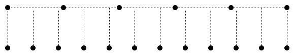
False :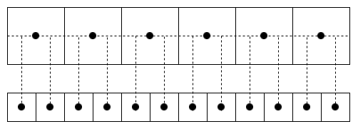
Therefore, we can see that the former here is more in line with our needs, because the implementation of the algorithms involving bilinear interpolation mentioned here (such as the previous deformable revolution) puts pixels on the vertices of the grid (according to this idea, it is more in line with the experimental phenomenon, which I will describe for the time being)
grid_sampled_shift = torch.cat(
    [
        F.grid_sample(
            x,
            torch.cat(
                [
                    2 * torch.clamp(w_coord + w, 0, 4) / (5 - 1) - 1,
                    2 * torch.clamp(h_coord + h, 0, 4) / (5 - 1) - 1,
                ],
                dim=-1,
            ),
            mode="bilinear",
            align_corners=True,
        )
        for x, (h, w) in zip(x.chunk(4, dim=1), [(0, -1), (0, 1), (-1, 0), (1, 0)])
    ],
    dim=1,
)
print(grid_sampled_shift)

'''
tensor([[[[0., 0., 0., 0., 0.],
          [1., 1., 1., 1., 1.],
          [2., 2., 2., 2., 2.],
          [3., 3., 3., 3., 3.],
          [4., 4., 4., 4., 4.]],

         [[0., 0., 1., 2., 3.],
          [0., 0., 1., 2., 3.],
          [0., 0., 1., 2., 3.],
          [0., 0., 1., 2., 3.],
          [0., 0., 1., 2., 3.]],

         [[0., 0., 0., 0., 0.],
          [1., 1., 1., 1., 1.],
          [2., 2., 2., 2., 2.],
          [3., 3., 3., 3., 3.],
          [4., 4., 4., 4., 4.]],

         [[1., 2., 3., 4., 4.],
          [1., 2., 3., 4., 4.],
          [1., 2., 3., 4., 4.],
          [1., 2., 3., 4., 4.],
          [1., 2., 3., 4., 4.]],

         [[0., 0., 0., 0., 0.],
          [0., 0., 0., 0., 0.],
          [1., 1., 1., 1., 1.],
          [2., 2., 2., 2., 2.],
          [3., 3., 3., 3., 3.]],

         [[0., 1., 2., 3., 4.],
          [0., 1., 2., 3., 4.],
          [0., 1., 2., 3., 4.],
          [0., 1., 2., 3., 4.],
          [0., 1., 2., 3., 4.]],

         [[1., 1., 1., 1., 1.],
          [2., 2., 2., 2., 2.],
          [3., 3., 3., 3., 3.],
          [4., 4., 4., 4., 4.],
          [4., 4., 4., 4., 4.]],

         [[0., 1., 2., 3., 4.],
          [0., 1., 2., 3., 4.],
          [0., 1., 2., 3., 4.],
          [0., 1., 2., 3., 4.],
          [0., 1., 2., 3., 4.]]]])
'''
Some other thoughts
About f.grid_ Error problem of sample
Due to F.grid_sample involves normalization operation, which naturally leads to precision loss
So in fact, this method is not recommended if you want to achieve accurate control
If the position is just on the corner of the cell, the nearest neighbor interpolation mode can be used to obtain a more neat result
Here is an example:
h_coord, w_coord = torch.meshgrid(torch.arange(7), torch.arange(7))
h_coord = h_coord.reshape(1, 7, 7, 1)
w_coord = w_coord.reshape(1, 7, 7, 1)
grid = torch.cat(
    [
        2 * torch.clamp(w_coord, 0, 6) / (7 - 1) - 1,
        2 * torch.clamp(h_coord, 0, 6) / (7 - 1) - 1,
    ],
    dim=-1,
)
print(grid)
print(pad_x[:, :2])

print("mode=bilinear\n", F.grid_sample(pad_x[:, :2], grid, mode="bilinear", align_corners=True))
print("mode=nearest\n", F.grid_sample(pad_x[:, :2], grid, mode="nearest", align_corners=True))

'''
tensor([[[[-1.0000, -1.0000],
          [-0.6667, -1.0000],
          [-0.3333, -1.0000],
          [ 0.0000, -1.0000],
          [ 0.3333, -1.0000],
          [ 0.6667, -1.0000],
          [ 1.0000, -1.0000]],

         [[-1.0000, -0.6667],
          [-0.6667, -0.6667],
          [-0.3333, -0.6667],
          [ 0.0000, -0.6667],
          [ 0.3333, -0.6667],
          [ 0.6667, -0.6667],
          [ 1.0000, -0.6667]],

         [[-1.0000, -0.3333],
          [-0.6667, -0.3333],
          [-0.3333, -0.3333],
          [ 0.0000, -0.3333],
          [ 0.3333, -0.3333],
          [ 0.6667, -0.3333],
          [ 1.0000, -0.3333]],

         [[-1.0000,  0.0000],
          [-0.6667,  0.0000],
          [-0.3333,  0.0000],
          [ 0.0000,  0.0000],
          [ 0.3333,  0.0000],
          [ 0.6667,  0.0000],
          [ 1.0000,  0.0000]],

         [[-1.0000,  0.3333],
          [-0.6667,  0.3333],
          [-0.3333,  0.3333],
          [ 0.0000,  0.3333],
          [ 0.3333,  0.3333],
          [ 0.6667,  0.3333],
          [ 1.0000,  0.3333]],

         [[-1.0000,  0.6667],
          [-0.6667,  0.6667],
          [-0.3333,  0.6667],
          [ 0.0000,  0.6667],
          [ 0.3333,  0.6667],
          [ 0.6667,  0.6667],
          [ 1.0000,  0.6667]],

         [[-1.0000,  1.0000],
          [-0.6667,  1.0000],
          [-0.3333,  1.0000],
          [ 0.0000,  1.0000],
          [ 0.3333,  1.0000],
          [ 0.6667,  1.0000],
          [ 1.0000,  1.0000]]]])
tensor([[[[0., 0., 0., 0., 0., 0., 0.],
          [0., 0., 0., 0., 0., 0., 0.],
          [1., 1., 1., 1., 1., 1., 1.],
          [2., 2., 2., 2., 2., 2., 2.],
          [3., 3., 3., 3., 3., 3., 3.],
          [4., 4., 4., 4., 4., 4., 4.],
          [4., 4., 4., 4., 4., 4., 4.]],

         [[0., 0., 1., 2., 3., 4., 4.],
          [0., 0., 1., 2., 3., 4., 4.],
          [0., 0., 1., 2., 3., 4., 4.],
          [0., 0., 1., 2., 3., 4., 4.],
          [0., 0., 1., 2., 3., 4., 4.],
          [0., 0., 1., 2., 3., 4., 4.],
          [0., 0., 1., 2., 3., 4., 4.]]]])
mode=bilinear
 tensor([[[[0.0000e+00, 0.0000e+00, 0.0000e+00, 0.0000e+00, 0.0000e+00,
           0.0000e+00, 0.0000e+00],
          [1.1921e-07, 1.1921e-07, 1.1921e-07, 1.1921e-07, 1.1921e-07,
           1.1921e-07, 1.1921e-07],
          [1.0000e+00, 1.0000e+00, 1.0000e+00, 1.0000e+00, 1.0000e+00,
           1.0000e+00, 1.0000e+00],
          [2.0000e+00, 2.0000e+00, 2.0000e+00, 2.0000e+00, 2.0000e+00,
           2.0000e+00, 2.0000e+00],
          [3.0000e+00, 3.0000e+00, 3.0000e+00, 3.0000e+00, 3.0000e+00,
           3.0000e+00, 3.0000e+00],
          [4.0000e+00, 4.0000e+00, 4.0000e+00, 4.0000e+00, 4.0000e+00,
           4.0000e+00, 4.0000e+00],
          [4.0000e+00, 4.0000e+00, 4.0000e+00, 4.0000e+00, 4.0000e+00,
           4.0000e+00, 4.0000e+00]],

         [[0.0000e+00, 1.1921e-07, 1.0000e+00, 2.0000e+00, 3.0000e+00,
           4.0000e+00, 4.0000e+00],
          [0.0000e+00, 1.1921e-07, 1.0000e+00, 2.0000e+00, 3.0000e+00,
           4.0000e+00, 4.0000e+00],
          [0.0000e+00, 1.1921e-07, 1.0000e+00, 2.0000e+00, 3.0000e+00,
           4.0000e+00, 4.0000e+00],
          [0.0000e+00, 1.1921e-07, 1.0000e+00, 2.0000e+00, 3.0000e+00,
           4.0000e+00, 4.0000e+00],
          [0.0000e+00, 1.1921e-07, 1.0000e+00, 2.0000e+00, 3.0000e+00,
           4.0000e+00, 4.0000e+00],
          [0.0000e+00, 1.1921e-07, 1.0000e+00, 2.0000e+00, 3.0000e+00,
           4.0000e+00, 4.0000e+00],
          [0.0000e+00, 1.1921e-07, 1.0000e+00, 2.0000e+00, 3.0000e+00,
           4.0000e+00, 4.0000e+00]]]])
mode=nearest
 tensor([[[[0., 0., 0., 0., 0., 0., 0.],
          [0., 0., 0., 0., 0., 0., 0.],
          [1., 1., 1., 1., 1., 1., 1.],
          [2., 2., 2., 2., 2., 2., 2.],
          [3., 3., 3., 3., 3., 3., 3.],
          [4., 4., 4., 4., 4., 4., 4.],
          [4., 4., 4., 4., 4., 4., 4.]],

         [[0., 0., 1., 2., 3., 4., 4.],
          [0., 0., 1., 2., 3., 4., 4.],
          [0., 0., 1., 2., 3., 4., 4.],
          [0., 0., 1., 2., 3., 4., 4.],
          [0., 0., 1., 2., 3., 4., 4.],
          [0., 0., 1., 2., 3., 4., 4.],
          [0., 0., 1., 2., 3., 4., 4.]]]])
'''
F.grid_ Relationship between sample and deformable revolution
Although they both realize the adjustment of the mapping relationship between input and output positions, there are obvious differences between them
Different reference coordinate systems
- The coordinate system of the former is a normalized coordinate system based on the overall input. The origin is the central position of the input HW plane, and the H axis and W axis are in the downward and right directions respectively In the coordinate system WOH, the upper left corner of the input data is $(- 1, - 1) $, and the upper right corner is $(1, - 1) $
- The latter coordinate system is relative to the initial action position of the weight But in fact, it is actually understood here as along the H axis and the w axis_ Relative offset_ More appropriate For example, if the weight action position is shifted to the left by one unit, the corresponding offset parameter group $(\ delta_h, \delta_w) $can be taken as $(0, - 1) $, that is, the $W $coordinate of the action position relative to the original action position plus a $- 1 $
Different effects
- The former directly adjusts the coordinates of the overall input, and has the same adjustment effect for all input channels
- Because the latter is built on convolution operation, it is more convenient to deal with different offset_groups and different local areas that may actually overlap (kernel_height * kernel_width) Therefore, the actual function is more flexible and adjustable
The second spring of Shift operation
Although many forms of spatial shift operation have been explored in previous work, they have not attracted much attention
- (CVPR 2018) [Grouped Shift] Shift: A Zero FLOP, Zero Parameter Alternative to Spatial Convolutions:
- (ICCV 2019) 4-Connected Shift Residual Networks
- (NIPS 2018) [Active Shift] Constructing Fast Network through Deconstruction of Convolution
- (CVPR 2019) [Sparse Shift] All You Need Is a Few Shifts: Designing Efficient Convolutional Neural Networks for Image Classification
Most of these works focus on the design of lightweight networks, and now these shift based methods combine the clipper MLP, which seems to have aroused some new splashes
The current methods often adopt more effective training settings, and the strategies outside these models also greatly improve the performance of the model to a certain extent In fact, it will also make people wonder. If the shift operations before migration are directly transferred to the MLP framework here, perhaps the performance will not be poor?
In fact, this idea is also applicable to the traditional CNN method. If the previous structures use the same training strategy, how much can they be worse than now? It is estimated that only those big men who have cards, time and patience can explore it
In fact, on the whole, the existing MLP methods based on spatial offset can be regarded as [(NIPS 2018) [active shift] constructing fast network through deconstruction of revolution]( https://www.yuque.com/lart/ar... )A specialized version of the work
In other words, the offset parameters of adaptive learning in this work are changed to fixed offset parameters