The first two blogs retrieve information about python data analysis in the Label (tab) https://www.cnblogs.com/lyuzt/p/10636501.html ) and visual analysis of the acquired data ( https://www.cnblogs.com/lyuzt/p/10643941.html This time, we use sklearn to make a simple salary forecast for python data analysts with different academic qualifications and work experience.Now that you have an overview of the dataset in the previous two blogs, you can get directly to the topic.

1. Conversion of pay

Before that, import the module and read in the file, not only the training data file, but also a set of self-designed test data files.

import pandas as pd
import numpy as np
import matplotlib.pyplot as plt

train_file = "analyst.csv"
test_file = "test.csv"
# Read file to get data
train_data = pd.read_csv(train_file, encoding="gbk")
train_data = train_data.drop('ID', axis=1)

test_data = pd.read_csv(test_file, encoding="gbk")
train_data.shape, test_data.shape

For better analysis, we need to preprocess the salary.Because of its scattered distribution, the number of many values is only 1.For the sake of not causing too much error, it can be divided into [less than 5k, 5k-10k, 10k-20k, 20k-30k, 30k-40k, 40K or more] according to its distribution. For the sake of more convenient analysis, the median of each salary range is taken and divided into the ranges we specify.

salarys = train_data['salary'].unique()     # Get different values for salary
for salary in salarys:
    # according to'-'Divide and remove'k',Convert values at each end to integers
    min_sa = int(salary.split('-')[0][:-1])
    max_sa = int(salary.split('-')[1][:-1])
    # median
    median_sa = (min_sa + max_sa) / 2
    # Judges its value and divides it into specified ranges
    if median_sa < 5:
        train_data.replace(salary, '5k Following', inplace=True)
    elif median_sa >= 5 and median_sa < 10:
        train_data.replace(salary, '5k-10k', inplace=True)
    elif median_sa >= 10 and median_sa < 20:
        train_data.replace(salary, '10k-20k', inplace=True)
    elif median_sa >= 20 and median_sa < 30:
        train_data.replace(salary, '20k-30k', inplace=True)
    elif median_sa >= 30 and median_sa < 40:
        train_data.replace(salary, '30k-40k', inplace=True)
    else:
        train_data.replace(salary, '40k Above', inplace=True)

Once the process is complete, we can extract the "salary" separately as a label for the training set.

y_train = train_data.pop('salary').values

 

2. Converting variables

Converts a category variable into a numeric expression

Since variables are not numeric variables, the computer cannot recognize them during training, so they need to be converted.When we use numerical s to express categorical s, it is important to note that numbers have their own meaning, so using them indiscriminately can cause difficulties for subsequent model learning.So we can use One-Hot to represent categories.

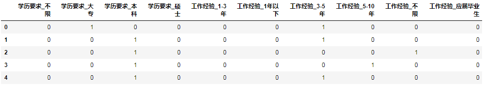
The get_dummies method that comes with pandas can do One-Hot with one click.Here's how I understand One-Hot: for example, data ['academic qualifications'] has'junior college','undergraduate','master','unlimited'.However, data ['academic qualifications']=='undergraduate', he can be expressed as {'college': 0,'undergraduate': 1,'master': 0,'unlimited': 0} in a dictionary, expressed as [0, 1, 0, 0] in a vector.

Before that, it was a little easier to combine the test set with the training set.

data = pd.concat((train_data, test_data), axis=0)
dummied_data = pd.get_dummies(data)
dummied_data.head()

In order to better understand One-Hot, the results after processing are shown as follows:

  

Of course, there are other ways to do this, such as replacing different values with numbers.

The last time you did a visual analysis, you already knew there were no missing values in the dataset. To follow the process and ensure correctness, check again to see if there are any missing values.

dummied_data.isnull().sum().sort_values(ascending=False).head(10)

　　        　　

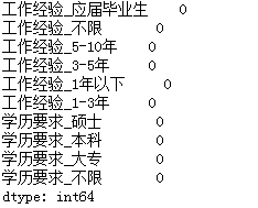
OK, good, no missing values.These values are simple and don't require much work, but first separate the training set from the test set.

X_train = dummied_data[:train_data.shape[0]].values
X_test = dummied_data[-test_data.shape[0]:].values

 

3. Selection of parameters

1. Decision Tree

from sklearn.tree import DecisionTreeClassifier
from sklearn.model_selection import cross_val_score
features_scores = []
max_features = [.1, .2, .3, .4, .5, .6, .7, .8, .9]
for max_feature in max_features:
    clf = DecisionTreeClassifier(max_features=max_feature)
    features_score = cross_val_score(clf, X_train, y_train, cv=5)
    features_scores.append(np.mean(features_score))
plt.plot(max_features, features_scores)

This process mainly obtains the parameters to make the model better through cross-validation, which can be roughly understood as dividing the training set into several parts, then setting them as training set and test set respectively, and averaging the results from repeated cyclic training.Emmm... Feels like it's a bit general, or you can look it up on the Internet in more detail.

The parameters and values we get are shown in the figure:

　　　　　　　　　　

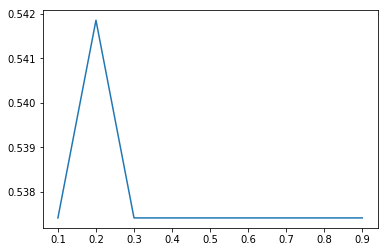
Visible when max_features = 0.2 reaches the maximum, about 0.5418.

2. ensemble (integrated algorithm)

Integrated learning simply means predicting datasets with multiple classifiers to improve the generalization ability of the overall classifier.Here, sklearn's AdaBoostClassifier (adaptive boosting) is used to learn multiple classifiers by changing the weights of training samples, and to linearly combine them to improve generalization performance.

from sklearn.ensemble import AdaBoostClassifier
n_scores = []
estimator_nums = [5, 10, 15, 20, 25, 30, 35, 40]
for estimator_num in estimator_nums:
    clf = AdaBoostClassifier(n_estimators=estimator_num, base_estimator=dtc)
    n_score = cross_val_score(clf, X_train, y_train, cv=5)
    n_scores.append(np.mean(n_score))
plt.plot(estimator_nums, n_scores)

　　　　　　　　　　

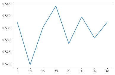
When estimators=20, the score is the highest, about 0.544, and although it is not much different from the score of a single decision tree, it is generally higher.

4. Modeling

Once you have selected the parameters, you are ready to build your model.

dtc = DecisionTreeClassifier(max_features=0.2)
abc = AdaBoostClassifier(n_estimators=20)
# train
abc.fit(X_train, y_train)
dtc.fit(X_train, y_train)
# Forecast
y_dtc = dtc.predict(X_test)
y_abc = abc.predict(X_test)

test_data['salary(Single Decision Tree)'] = y_dtc
test_data['salary(boosting)'] = y_abc

　        　

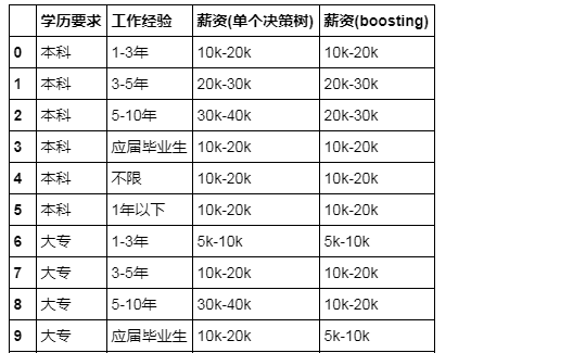
As for results, it is impossible to predict perfectly, and the results of different models will vary, and it remains to be debated whether the predicted results conform to common sense, so just treat them as a small project with the specific code here: https://github.com/MaxLyu/Lagou_Analyze