1, What is TensorFlow

TensorFlow is a powerful open source software library developed by Google Brain team for deep neural network (DNN). It was first released in November 2015 and is available under the Apache 2.x protocol license. Up to now, in just two years, about 845 contributors of its GitHub library have submitted more than 17000 times, which in itself is an indicator of TensorFlow popularity and performance.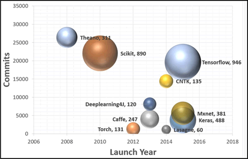

Open source deep learning library TensorFlow allows the calculation of deep neural network to be deployed to any number of CPU or GPU servers, PC s or mobile devices, and only uses one TensorFlow API. You may ask, there are many other deep learning libraries, such as Torch. Theano. Caffe and MxNet. What's the difference between TensorFlow and other deep learning libraries? Most deep learning libraries, including TensorFlow, can automatically derive, open source, support multiple CPUs / GPUs, have pre training models, and support common NN architectures, such as recurrent neural network (RNN), convolutional neural network (CNN) and deep confidence network (DBN).
TensorFlow has more features, as follows:
a. Support for all popular languages, such as Python. C++. Java. R and Go.
b. It can work on multiple platforms, even mobile platforms and distributed platforms.
c. It is supported by all cloud services (AWS. Google and Azure).
d. Keras – advanced neural network API, has been integrated with TensorFlow.
e. Compared with Torch/Theano, TensorFlow has better visualization of calculation chart.
f. Allows the model to be deployed to industrial production and is easy to use.
g. Very good community support.
h. TensorFlow is not only a software library, but also a set of software including TensorFlow, TensorBoard and TensorServing.

2, hello world

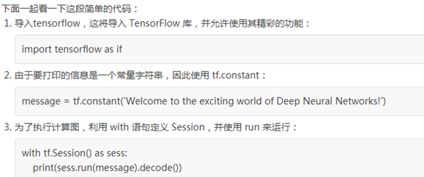
The first program to learn in any computer language is hello world, starting with the program Hello world.
Code for TensorFlow installation verification:

import tensorflow as tf 
message = tf .constant ( 'Welcome to the exciting world of Deep Neural Networks! ')
with tf .Session () as sess :
print (sess. run (message) .decode() )

Report errors:
Could not load dynamic library 'cudart64_101.dll'; dlerror: cudart64_101.dll not found. Ignore above cudart dlerror if you do not have a GPU set up on your machine.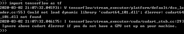

When GPU cannot run, it will return to CPU version.
Attempting to fetch value instead of handling error internal: could not retrieve CUDA device attribute <81: UNKNOWN ERROR<1>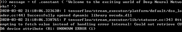

Video card memory too many times..

Install TensorFlow CPU version: PIP3 install TensorFlow CPU - I https://pypi.double.com/simple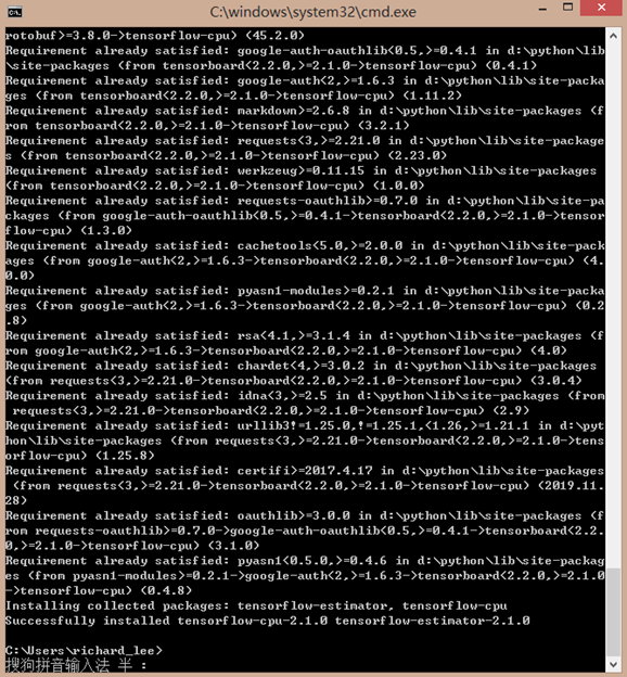

Test whether TensorFlow is installed successfully

import tensorflow as tf
version = tf.__version__
gpu_ok = tf.test.is_gpu_available()
print("tf version:",version,"\nif use GPU",gpu_ok)

The results are as follows: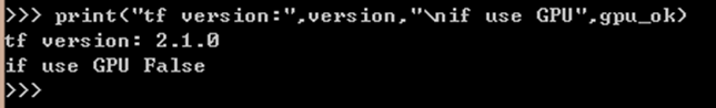

Run again, problem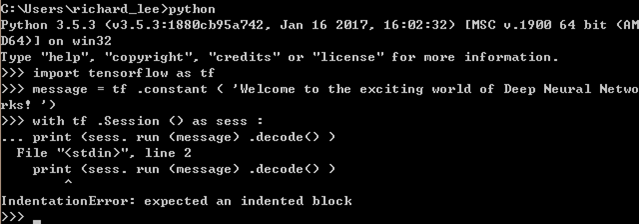

Solution:
It's ok to add a space in front of the logic code for error reporting. An indentation solves the exception. Solving the bug is not the main purpose. Understanding the syntax structure and characteristics of python is what we should do.
In python, method bodies are not distinguished by {}. In python, syntax logic blocks are identified by indentation (i.e. if, while, for, def, etc.). In python, all logical code blocks, that is, the code in a method, must use the same indentation to identify that the distinction is the same method, or the compilation will report an error. The so-called indentation is the blank at the beginning of each line. This white space can consist of multiple spaces or tabs. You can indent any way in python. For example, three spaces and two tabs are legal. But the same must be used under the same logical block.

3, A simple TensorFlow program

1. Create a new python file of linear fitting, the content of which is as follows:

import tensorflow as tf
X = tf.constant([[1.0, 2.0, 3.0], [4.0, 5.0, 6.0]])
y = tf.constant([[10.0], [20.0]])
class Linear(tf.keras.Model):
    def __init__(self):
        super().__init__()
        self.dense = tf.keras.layers.Dense(
            units=1,
            activation=None,
            kernel_initializer=tf.zeros_initializer(),
            bias_initializer=tf.zeros_initializer()
        )
    def call(self, input):
        output = self.dense(input)
        return output

model = Linear()
optimizer = tf.keras.optimizers.SGD(learning_rate=0.01)
for i in range(100):
    with tf.GradientTape() as tape:
        y_pred = model(X)      # Call model y ﹣ PRED = model (x) instead of explicitly writing out y ﹣ PRED = a * x + B
        loss = tf.reduce_mean(tf.square(y_pred - y))
    grads = tape.gradient(loss, model.variables)    # Use the attribute model.variables to get all the variables in the model directly
    optimizer.apply_gradients(grads_and_vars=zip(grads, model.variables))
    if i % 10 == 0:
        print(i, loss.numpy())
print(model.variables)

1. Then run, and the result is as follows

4, Image classification

We will build a simple image classifier

from __future__ import absolute_import, division, print_function
import tensorflow as tf
from tensorflow import keras
from tensorflow.keras import layers
import matplotlib.pyplot as plt
import numpy as np
print(tf.__version__)

1. Get Fashion MNIST data set

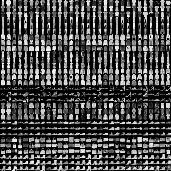
Use the Fashion MNIST dataset, which contains 70000 grayscale images in 10 categories.

mnist=keras.datasets.mnist
(train_images, train_labels), (test_images, test_labels) = keras.datasets.fashion_mnist.load_data()

class_names = ['T-shirt/top', 'Trouser', 'Pullover', 'Dress', 'Coat', 
               'Sandal', 'Shirt', 'Sneaker', 'Bag', 'Ankle boot']

2. Explore data

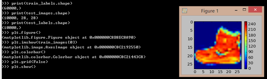
Explore the format of the dataset before training the model. There are 60000 images in the following display training set, each of which is represented as 28 x 28 pixels:

print(train_images.shape)
print(train_labels.shape)
print(test_images.shape)
print(test_labels.shape)

3. Processing data

plt.figure()
plt.imshow(train_images[0])
plt.colorbar()
plt.grid(False)
plt.show()

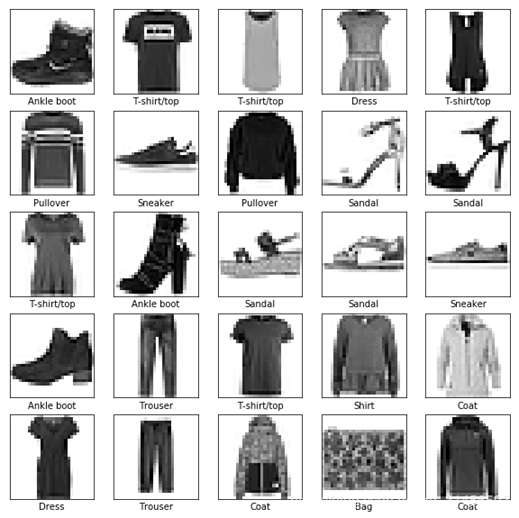
train_images = train_images / 255.0
test_images = test_images / 255.0
plt.figure(figsize=(10,10))
for i in range(25):
    plt.subplot(5,5,i+1)
    plt.xticks([])
    plt.yticks([])
    plt.grid(False)
    plt.imshow(train_images[i], cmap=plt.cm.binary)
    plt.xlabel(class_names[train_labels[i]])
    plt.show()

4. Network construction

model = keras.Sequential(
[
    layers.Flatten(input_shape=[28, 28]),
    layers.Dense(128, activation='relu'),
    layers.Dense(10, activation='softmax')
])

model.compile(optimizer='adam',
             loss='sparse_categorical_crossentropy',
             metrics=['accuracy'])

5. Training and verification

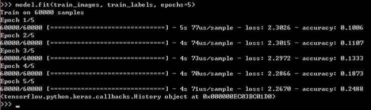
model.fit(train_images, train_labels, epochs=5)

model.evaluate(test_images, test_labels)

6. forecast

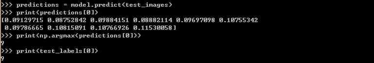
predictions = model.predict(test_images)
print(predictions[0])
print(np.argmax(predictions[0]))
print(test_labels[0])

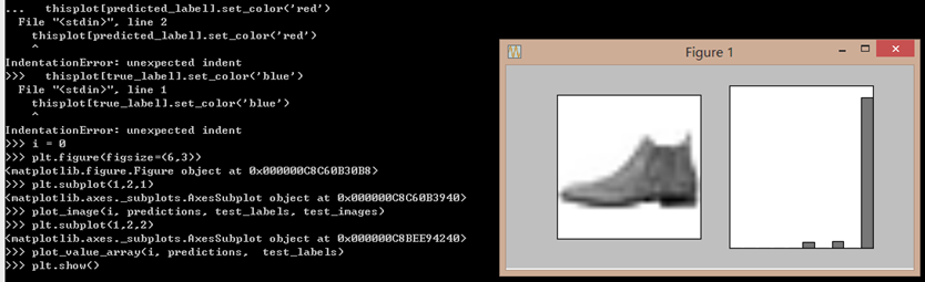
def plot_image(i, predictions_array, true_label, img):
  predictions_array, true_label, img = predictions_array[i], true_label[i], img[i]
  plt.grid(False)
  plt.xticks([])
  plt.yticks([])
  plt.imshow(img, cmap=plt.cm.binary)

  predicted_label = np.argmax(predictions_array)
  if predicted_label == true_label:
    color = 'blue'
  else:
    color = 'red'
  
  plt.xlabel("{} {:2.0f}% ({})".format(class_names[predicted_label],
                                100*np.max(predictions_array),
                                class_names[true_label]),
                                color=color)

def plot_value_array(i, predictions_array, true_label):
  predictions_array, true_label = predictions_array[i], true_label[i]
  plt.grid(False)
  plt.xticks([])
  plt.yticks([])
  thisplot = plt.bar(range(10), predictions_array, color="#777777")
  plt.ylim([0, 1]) 
  predicted_label = np.argmax(predictions_array)
 
  thisplot[predicted_label].set_color('red')
  thisplot[true_label].set_color('blue')
i = 0
plt.figure(figsize=(6,3))
plt.subplot(1,2,1)
plot_image(i, predictions, test_labels, test_images)
plt.subplot(1,2,2)
plot_value_array(i, predictions,  test_labels)
plt.show()

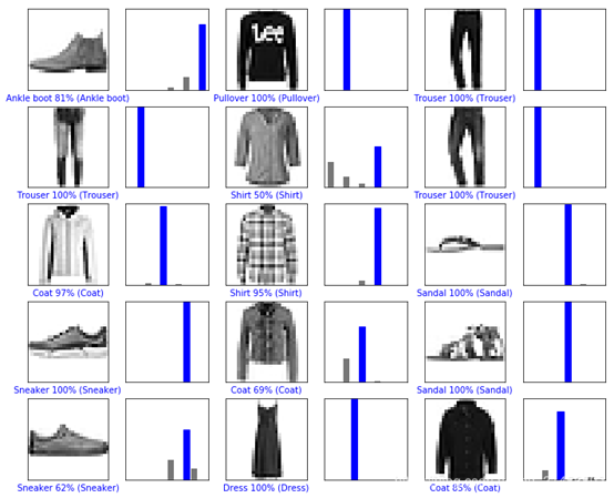
# Plot the first X test images, their predicted label, and the true label
# Color correct predictions in blue, incorrect predictions in red
num_rows = 5
num_cols = 3
num_images = num_rows*num_cols
plt.figure(figsize=(2*2*num_cols, 2*num_rows))
for i in range(num_images):
  plt.subplot(num_rows, 2*num_cols, 2*i+1)
  plot_image(i, predictions, test_labels, test_images)
  plt.subplot(num_rows, 2*num_cols, 2*i+2)
  plot_value_array(i, predictions, test_labels)
  plt.show()

[1]: https://blog.csdn.net/qq_31456593/article/details/88605746
[2]: http://c.biancheng.net/view/1882.html