Vectorization of code means that the problem to be solved is vectorized in essence. It only needs some numpy skills to make the code run faster, but vectorization is not very easy.
Vectorization code example: game of life
The universe of life game is a two-dimensional orthogonal grid. Each grid (cell) is in two possible states, life or death. Each cell located in a grid interacts with its eight adjacent cells (horizontally, vertically or diagonally adjacent cells). In each evolutionary step, the following transformations occur:
- The living cells of less than two neighbors will die.
- The living cells of more than three neighbors will die.
- Living cells with two or three neighbors survive and can be maintained until the next generation.
- There happened to be the resurrection of the dead cells of three living cell neighbors
Python implementation
The grid uses a two-dimensional list to represent the initial state of the system, 1 for survival and 0 for death.
Z = [[0,0,0,0,0,0],
     [0,0,0,1,0,0],
     [0,1,0,1,0,0],
     [0,0,1,1,0,0],
     [0,0,0,0,0,0],
     [0,0,0,0,0,0]]
To simplify the calculation, all boundaries are set to 0. First, define a function to count the number of living cells adjacent to each grid (the grid without boundary is not calculated).
def compute_neighbours(Z):
    shape = len(Z), len(Z[0])
    N  = [[0,]*(shape[0]) for i in range(shape[1])]
    # Traverse each element, the lattice without boundary, and calculate the sum of surrounding elements
    for x in range(1,shape[0]-1):
        for y in range(1,shape[1]-1):
            N[x][y] = Z[x-1][y-1]+Z[x][y-1]+Z[x+1][y-1] \
                    + Z[x-1][y]            +Z[x+1][y]   \
                    + Z[x-1][y+1]+Z[x][y+1]+Z[x+1][y+1]
    return N
# Test the statistics compute_neighbours(Z) out: [[0, 0, 0, 0, 0, 0], [0, 1, 3, 1, 2, 0], [0, 1, 5, 3, 3, 0], [0, 2, 3, 2, 2, 0], [0, 1, 2, 2, 1, 0], [0, 0, 0, 0, 0, 0]]
Define the iteration function and carry out the next iteration according to the above four rules.
def iterate(Z):
    shape = len(Z), len(Z[0])
    N = compute_neighbours(Z) # Count the living cells of adjacent elements
    for x in range(1,shape[0]-1):
        for y in range(1,shape[1]-1):
             # If they are living cells and the number of living cells in their neighbors is less than 2 or more than 3, they will become dead cells
             if Z[x][y] == 1 and (N[x][y] < 2 or N[x][y] > 3):
                 Z[x][y] = 0
             # Otherwise, they are dead cells and the number of living cells in their neighbors is 3, which will turn into living cells
             elif Z[x][y] == 0 and N[x][y] == 3:
                 Z[x][y] = 1
    return Z
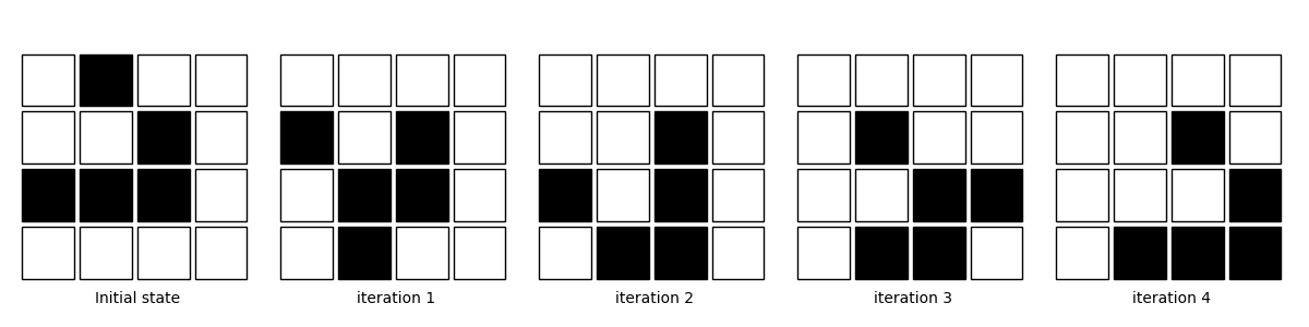
The following is the visualization result after 5 iterations (excluding boundary data)
Full code:
def compute_neighbours(Z):
    shape = len(Z), len(Z[0])
    N = [[0, ]*(shape[0]) for i in range(shape[1])]
    for x in range(1, shape[0]-1):
        for y in range(1, shape[1]-1):
            N[x][y] = Z[x-1][y-1]+Z[x][y-1]+Z[x+1][y-1] \
                    + Z[x-1][y]            +Z[x+1][y]   \
                    + Z[x-1][y+1]+Z[x][y+1]+Z[x+1][y+1]
    return N


def iterate(Z):
    shape = len(Z), len(Z[0])
    N = compute_neighbours(Z)
    for x in range(1, shape[0]-1):
        for y in range(1, shape[1]-1):
            if Z[x][y] == 1 and (N[x][y] < 2 or N[x][y] > 3):
                Z[x][y] = 0
            elif Z[x][y] == 0 and N[x][y] == 3:
                Z[x][y] = 1
    return Z

if __name__ == '__main__':
    import matplotlib.pyplot as plt
    from matplotlib.patches import Rectangle

    Z = [[0, 0, 0, 0, 0, 0],
         [0, 0, 0, 1, 0, 0],
         [0, 1, 0, 1, 0, 0],
         [0, 0, 1, 1, 0, 0],
         [0, 0, 0, 0, 0, 0],
         [0, 0, 0, 0, 0, 0]]

    figure = plt.figure(figsize=(12, 3))

    labels = ("Initial state",
              "iteration 1", "iteration 2",
              "iteration 3", "iteration 4")

    for i in range(5): # After 5 iterations
        ax = plt.subplot(1, 5, i+1, aspect=1, frameon=False)

        for x in range(1, 5):
            for y in range(1, 5):
                if Z[x][y] == 1:
                    facecolor = 'black' # Black represents survival
                else:
                    facecolor = 'white' # White represents death
                rect = Rectangle((x, 5-y), width=0.9, height=0.9,
                                 linewidth=1.0, edgecolor='black',
                                 facecolor=facecolor)
                ax.add_patch(rect)
        ax.set_xlim(.9, 5.1)
        ax.set_ylim(.9, 5.1)
        ax.set_xticks([])
        ax.set_yticks([])
        ax.set_xlabel(labels[i])

        for tick in ax.xaxis.get_major_ticks():
            tick.tick1On = tick.tick2On = False
        for tick in ax.yaxis.get_major_ticks():
            tick.tick1On = tick.tick2On = False

        iterate(Z)

    plt.tight_layout()
    plt.show()
Implementation of Numpy version
Observing the implementation of pure python version, nested loops are used to count the number of adjacent cells and iterative functions, which is inefficient, especially when calculating large-scale arrays. The main purpose of vectorization is to eliminate cyclic calculation as much as possible. Therefore, we first consider how to solve the problem of the number of adjacent cells through vectorization calculation.
The question is how to get all adjacent elements at once? For a one-dimensional array, the problem becomes how to obtain the left and right adjacent groups of elements at one time? As shown below:
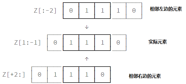
All left neighbors of each element (excluding boundary elements) are represented as Z[:-2], similarly, all right neighbors are represented as Z[2:]. Boundary elements are not considered here. To put it bluntly, the left neighbor of the left boundary or the right neighbor of the right boundary do not exist.
Extension of binary array:
Z = np.array(
[[0,0,0,0,0,0],
[0,0,0,1,0,0],
[0,1,0,1,0,0],
[0,0,1,1,0,0],
[0,0,0,0,0,0],
[0,0,0,0,0,0]]
)
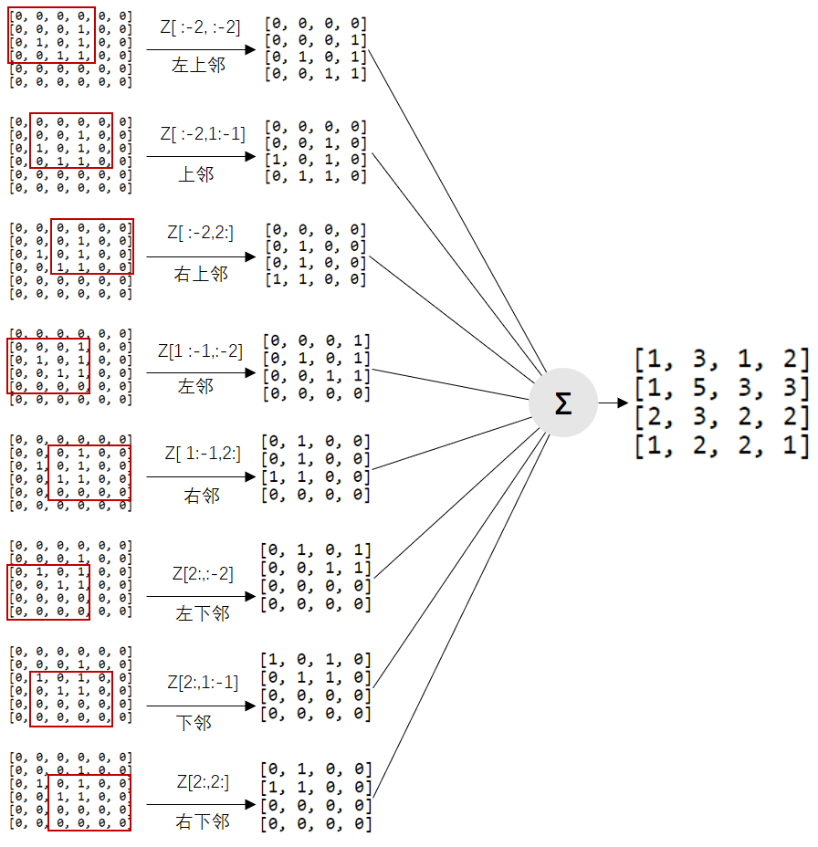
N = (
Z[ :-2, :-2] + Z[ :-2, 1:-1] + Z[ :-2, 2:] +
Z[1:-1, :-2] + Z[1:-1, 2:] +
Z[2: , :-2] + Z[2: , 1:-1] + Z[2: , 2:]
)
print(N)
out:
[[1 3 1 2]
[1 5 3 3]
[2 3 2 2]
[1 2 2 1]]The calculation result of nested loop is consistent with that of python version, but the boundary element is missing and needs to be supplemented. This is relatively simple in numpy and is completed with zeros assignment. The advantage of vectorization calculation is that nested loops are omitted and an addition is done.
Next, eliminate the loop in the iteration and turn the above four rules into numpy implementation.
# Implementation of numpy in the first version
# Flattened array
N_ = N.ravel()
Z_ = Z.ravel()

# Implementation rules
R1 = np.argwhere( (Z_==1) & (N_ < 2) )
R2 = np.argwhere( (Z_==1) & (N_ > 3) )
R3 = np.argwhere( (Z_==1) & ((N_==2) | (N_==3)) )
R4 = np.argwhere( (Z_==0) & (N_==3) )

# Assign values according to rules
Z_[R1] = 0
Z_[R2] = 0
Z_[R3] = Z_[R3]
Z_[R4] = 1

# Set boundary element to 0
Z[0,:] = Z[-1,:] = Z[:,0] = Z[:,-1] = 0
Although the first version of the implementation eliminates nested loops, four argwhere calls will lead to performance degradation. The alternative is to use the Boolean operation of numpy.
birth = (N==3)[1:-1,1:-1] & (Z[1:-1,1:-1]==0) # Resurrection conditions
survive = ((N==2) | (N==3))[1:-1,1:-1] & (Z[1:-1,1:-1]==1) # Survival conditions
Z[...] = 0 # Array zeroing
Z[1:-1,1:-1][birth | survive] = 1 # Set the elements that meet the survival conditions to 1
Based on the above optimization logic, increase the size of the array and observe the upgraded Game of life with animation
import numpy as np
import matplotlib.pyplot as plt
from matplotlib.animation import FuncAnimation


def update(*args):
    global Z, M

    N = (Z[0:-2, 0:-2] + Z[0:-2, 1:-1] + Z[0:-2, 2:] +
         Z[1:-1, 0:-2]                 + Z[1:-1, 2:] +
         Z[2:  , 0:-2] + Z[2:  , 1:-1] + Z[2:  , 2:])
    birth = (N == 3) & (Z[1:-1, 1:-1] == 0)
    survive = ((N == 2) | (N == 3)) & (Z[1:-1, 1:-1] == 1)
    Z[...] = 0
    Z[1:-1, 1:-1][birth | survive] = 1

    # Show past iterations
    M[M>0.25] = 0.25 # Threshold, which controls the gray value of display elements
    M *= 0.995 # Gray attenuation coefficient, which can be modified and observed by yourself
    M[Z==1] = 1
    im.set_data(M)


Z = np.random.randint(0, 2, (300, 600))
M = np.zeros(Z.shape)

size = np.array(Z.shape)
dpi = 80.0
figsize = size[1]/float(dpi), size[0]/float(dpi)
fig = plt.figure(figsize=figsize, dpi=dpi)
fig.add_axes([0.0, 0.0, 1.0, 1.0], frameon=False)
im = plt.imshow(M, interpolation='nearest', cmap=plt.cm.gray_r, vmin=0, vmax=1)
plt.xticks([]), plt.yticks([])

#matplotlib animation function, drawing function update, call interval 10ms,2000 frames end. Detailed parameter setting reference document
animation = FuncAnimation(fig, update, interval=10, frames=2000)
plt.show()