[translated from: Gradient Descent With RMSProp from Scratch]
[Note: Jason Brownlee likes PhD's articles very much, so he will do some translation and learning practice in his spare time. Here is the practice record of the corresponding work, hoping to help people in need!]
Gradient descent is an optimization algorithm, which follows the negative gradient of the objective function to locate the minimum value of the function.
One limitation of gradient descent is that it uses the same step size (learning rate) for each input variable. In short, AdaGrad is an extension of the gradient descent optimization algorithm, which allows the step size in each dimension used by the optimization algorithm to be automatically adjusted according to the gradient seen for the variable (partial derivative) during the search process.
One limitation of AdaGrad is that it may cause the step size of each parameter to be very small at the end of the search, which will greatly slow down the progress of the search and may mean that the optimal value cannot be found.
Root mean square propagation (or RMSProp) is an extension of the gradient descent method and the AdaGrad version of the gradient descent method. It uses the attenuation average of partial gradients to adapt to the step size of each parameter. The use of attenuated moving average allows the algorithm to forget the early gradient and focus on the recently observed partial gradient seen in the search process, overcoming the limitations of AdaGrad.
In this tutorial, you will learn how to use the RMSProp optimization algorithm to develop gradient descent from scratch. After completing this tutorial, you will learn:
Gradient descent is an optimization algorithm, which uses the gradient of the objective function to navigate the search space.
You can use the decaying moving average of the partial derivative (called RMSProp)Update gradient descent to use auto adaptive step size for each input variable.
How to implement from scratch RMSProp Optimize the algorithm and apply it to the objective function and evaluate the results.
Tutorial overview
This tutorial is divided into three parts; They are:
gradient descent
Root mean square propagation (RMSProp)
use RMSProp Gradient descent
    Two dimensional test questions
    use RMSProp Gradient descent optimization
    RMSProp Visual
gradient descent
Gradient descent is an optimization algorithm. It is technically called first-order optimization algorithm because it explicitly uses the first derivative of the objective function.
The first derivative, or "derivative" for short, is the rate of change or slope of the objective function at a specific point, such as for a specific input.
If the objective function accepts multiple input variables, it is called a multivariate function, and the input variable can be considered as a vector. Conversely, the derivative of multivariate objective function can also be used as a vector, which is generally called gradient.
Gradient: the first derivative of multivariate objective function.
For a particular input, the derivative or gradient points in the direction of the steepest rise of the objective function.
Gradient descent is a minimization optimization algorithm, which follows the negative number of the gradient descent of the objective function to locate the minimum value of the function. The gradient descent algorithm needs an objective function being optimized and the derivative function of the objective function. The objective function f() returns the fraction of a given input set, while the derivative function f '() gives the derivative of the objective function to a given input set. The gradient descent algorithm requires a starting point (x) in the problem, such as a randomly selected point in the input space. Then calculate the derivative and take a step in the input space, assuming that we are minimizing the objective function, which is expected to lead to the downhill motion in the objective function.
The downhill motion is carried out by first calculating the motion distance in the input space by multiplying the step size (called alpha or learning rate) by the slope. Then subtract it from the current point to make sure we move against the gradient or down the objective function.
x = x – step_size * f'(x)
The steeper the objective function of a given point is, the greater the amplitude of the gradient is. Conversely, the larger the step size in the search space is. The size of the step taken is scaled using the step super parameter.
Step size (alpha): a super parameter that controls how far the gradient moves in the search space for each iteration of the algorithm.
If the step size is too small, the movement in the search space will be very small and the search time will be very long. If the step size is too large, the search may bounce around the search space and skip the optimal value.
Now that we are familiar with the gradient descent optimization algorithm, let's take a look at RMSProp.
Root mean square propagation (RMSProp)
Root mean square propagation (RMSProp) is an extension of gradient descent optimization algorithm.
This is an unpublished extension, first described in Geoffrey Hinton's Coursera neural network course handout, especially topic 6e is "rmsprop: dividing the gradient by the operating average of the nearest amplitude".
RMSProp aims to accelerate the optimization process, such as reducing the number of function evaluations required to reach the optimal value, or improving the ability of the optimization algorithm, such as obtaining better final results. It is related to another extension of gradient descent, called adaptive gradient or AdaGrad.
AdaGrad aims to explore the idea of automatically customizing the step size (learning rate) for each parameter in the search space. This is achieved by first calculating the step size of a given dimension, and then moving on that dimension using the calculated step size and partial derivative. Then repeat this process for each dimension in the search space.
Adagrad calculates the step size of each parameter. First, sum the partial derivatives of the parameters seen during the search, and then divide the initial step super parameter by the square root of the square sum of the partial derivatives.
The custom step size of a parameter is calculated as follows:
cust_step_size = step_size / (1e-8 + sqrt(s))
Where cust_step_size is the calculation step of the input variable at a given point during the search, step_size is the initial step size, sqrt() is the square root operation, and s is the sum of the square partial derivatives of the input variables seen in the search process. This has the effect of smoothing the oscillations in search optimization problems, which have a large amount of curvature in the search space.
One problem with AdaGrad is that it slows down the search too much, resulting in a very small learning rate for each parameter or search dimension at the end of the run. This causes the search to stop prematurely before finding the minimum value.
RMSProp can be considered an extension of AdaGrad because it uses the decaying average or moving average of partial derivatives rather than the sum when calculating the learning rate of each parameter.
This is achieved by adding a new hyperparameter called rho, which acts like the momentum of partial derivative. Using the decaying moving average of partial derivatives allows the search to forget the early partial derivative values and focus on the recently seen shape of the search space.
The mean square partial derivative of a parameter is calculated as follows:
s(t+1) = (s(t) * rho) + (f'(x(t))^2 * (1.0-rho))
Where s(t+1) is the attenuation moving average of the square partial derivative of a parameter in the current iteration of the algorithm, s(t) is the attenuation moving average square partial derivative of the previous iteration, f '(x (T)) ^ 2 is the square partial derivative of the current parameter, and rho is a super parameter, usually 0.9 like momentum.
Since we are using the attenuation average of the partial derivative and calculating the square root of the average, we are naming the technology, such as the square root or root mean square (RMS) of the mean square partial derivative. For example, the custom step size of the parameter can be written as:
cust_step_size(t+1) = step_size / (1e-8 + RMS(s(t+1)))
Once we have the custom step of the parameter, we can update the parameter with the custom step and the partial derivative f'(x(t)).
x(t+1) = x(t) – cust_step_size(t+1) * f'(x(t))
This process is then repeated for each input variable until a new point is created in the search space and can be evaluated. RMSprop is a very effective extension of gradient descent and is one of the preferred methods for fitting deep learning neural networks. Now that we are familiar with the RMSprop algorithm, let's explore how to implement it and evaluate its performance.
Gradient descent using RMSProp
In this section, we will discuss how to use RMSProp algorithm to realize gradient descent optimization algorithm with adaptive gradient.
Two dimensional test questions
First, let's define an optimization function. We will use a simple two-dimensional function to square the input of each dimension and define a valid input range from - 1.0 to 1.0.
The following objective() function implements this function
# objective function
def objective(x, y):
	return x**2.0 + y**2.0
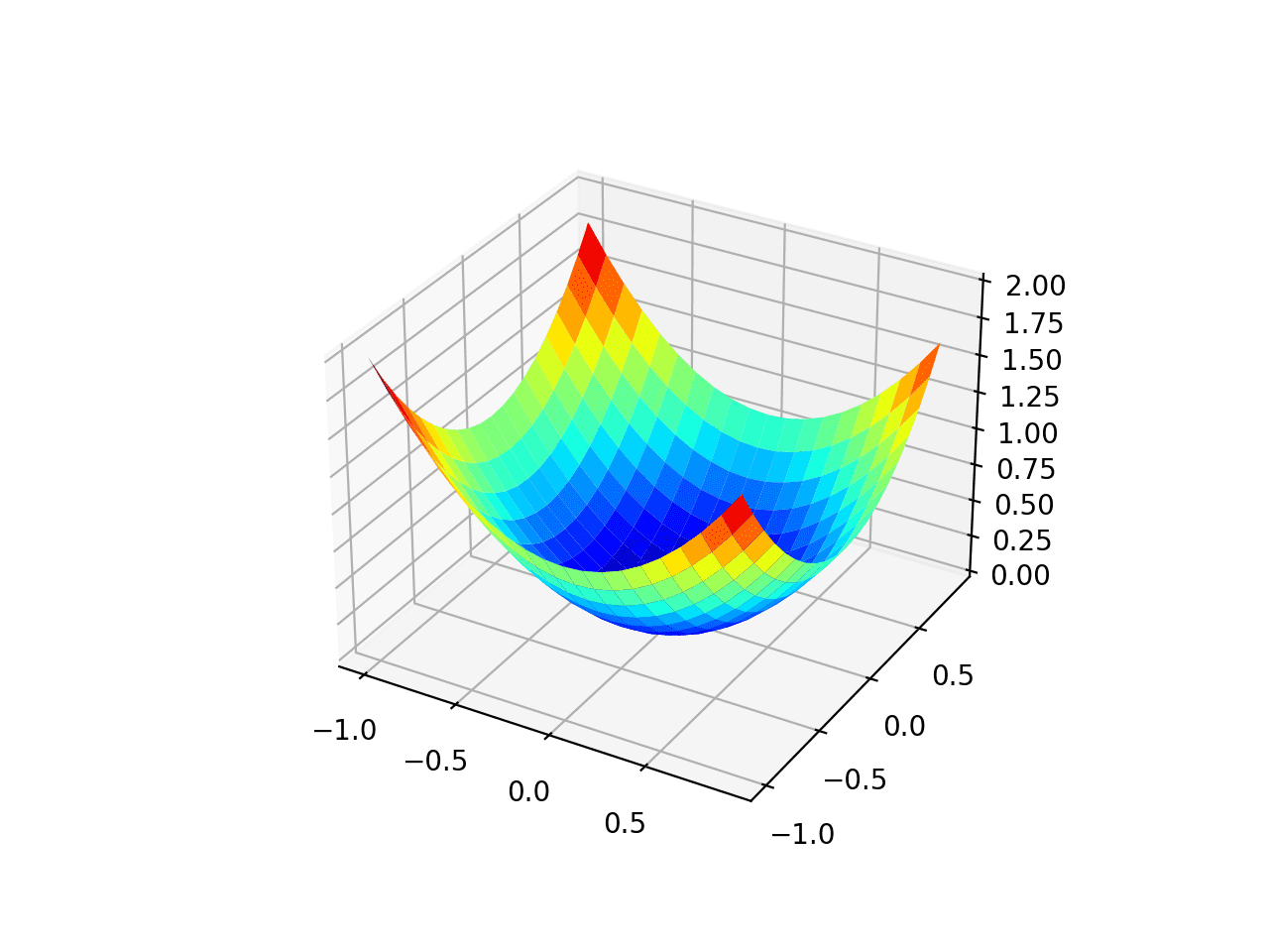
We can create a three-dimensional graph of the data set to feel the curvature of the response surface.
A complete example of drawing an objective function is listed below.
# 3d plot of the test function
from numpy import arange
from numpy import meshgrid
from matplotlib import pyplot

# objective function
def objective(x, y):
	return x**2.0 + y**2.0

# define range for input
r_min, r_max = -1.0, 1.0
# sample input range uniformly at 0.1 increments
xaxis = arange(r_min, r_max, 0.1)
yaxis = arange(r_min, r_max, 0.1)
# create a mesh from the axis
x, y = meshgrid(xaxis, yaxis)
# compute targets
results = objective(x, y)
# create a surface plot with the jet color scheme
figure = pyplot.figure()
axis = figure.gca(projection='3d')
axis.plot_surface(x, y, results, cmap='jet')
# show the plot
pyplot.show()
Run this example to create a 3D surface graph of the objective function.
We can see that the familiar bowl shape has a global minimum at f(0, 0) = 0.
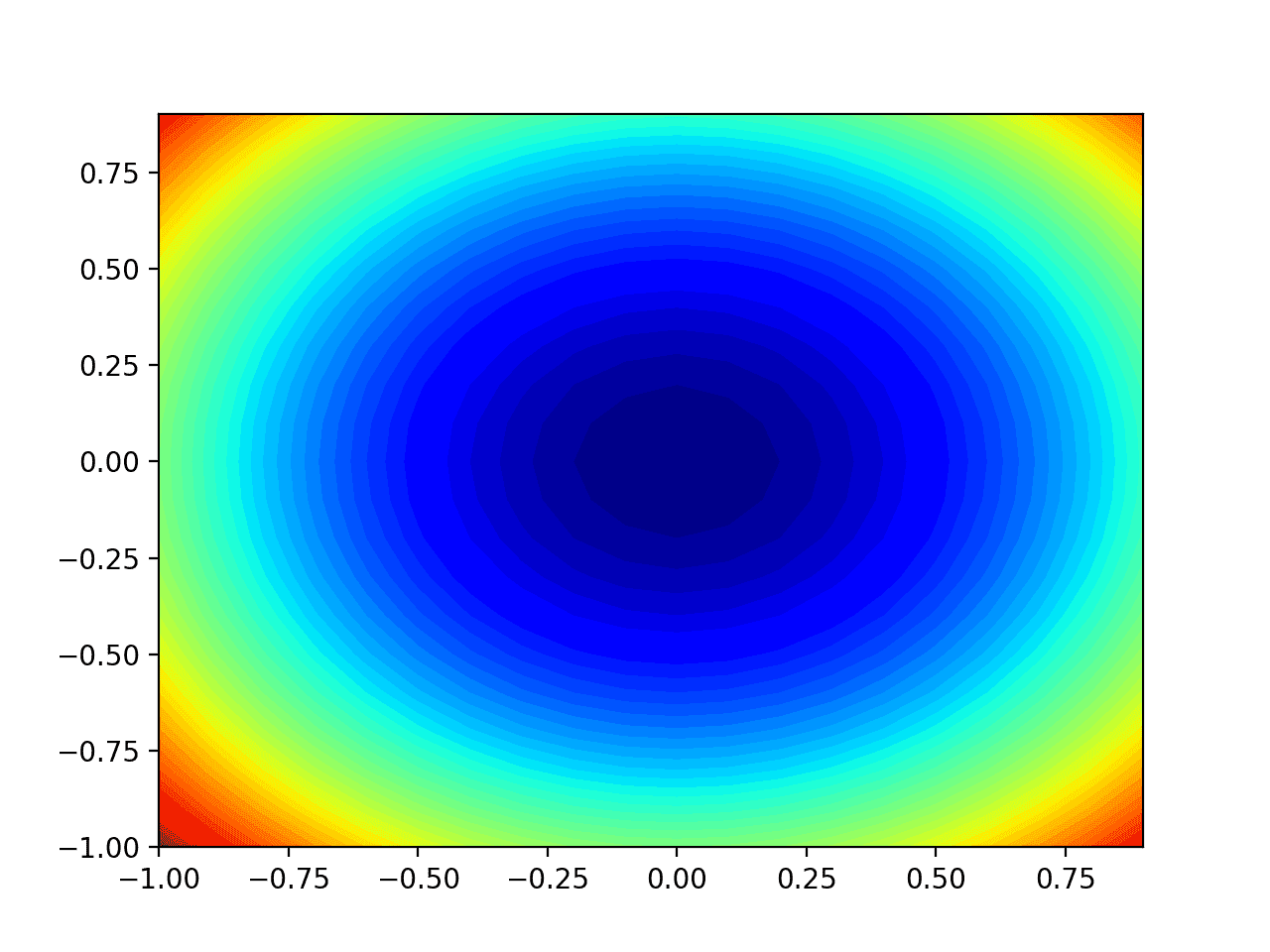
We can also create a two-dimensional diagram of the function. This will be helpful later when we want to draw the search progress.
The following example creates a contour map of the objective function.
# contour plot of the test function
from numpy import asarray
from numpy import arange
from numpy import meshgrid
from matplotlib import pyplot

# objective function
def objective(x, y):
	return x**2.0 + y**2.0

# define range for input
bounds = asarray([[-1.0, 1.0], [-1.0, 1.0]])
# sample input range uniformly at 0.1 increments
xaxis = arange(bounds[0,0], bounds[0,1], 0.1)
yaxis = arange(bounds[1,0], bounds[1,1], 0.1)
# create a mesh from the axis
x, y = meshgrid(xaxis, yaxis)
# compute targets
results = objective(x, y)
# create a filled contour plot with 50 levels and jet color scheme
pyplot.contourf(x, y, results, levels=50, cmap='jet')
# show the plot
pyplot.show()
Run this example to create a two-dimensional contour map of the objective function.
We can see that the shape of the bowl is compressed into an outline with a color gradient. We will use this graph to draw specific points explored during the search.
Now that we have a test objective function, let's see how to implement the RMSProp optimization algorithm.
Gradient descent optimization using RMSProp
We can apply the gradient descent of RMSProp to the test problem. First, we need a function to calculate the derivative of this function.
f(x) = x^2
f'(x) = x * 2
The derivative of x ^ 2 is x * 2 in each dimension. The derived () function implements this below.
# derivative of objective function
def derivative(x, y):
	return asarray([x * 2.0, y * 2.0])
Next, we can realize gradient descent optimization. First, we can select a random point within the scope of the problem as the starting point of the search. This assumes that we have an array that defines the search boundary. Each dimension has a row. The first column defines the minimum value and the second column defines the maximum value of the dimension.
# generate an initial point
solution = bounds[:, 0] + rand(len(bounds)) * (bounds[:, 1] - bounds[:, 0])
Next, we need to initialize the attenuation average of the square partial derivative of each dimension to 0.0.
# list of the average square gradients for each variable
sq_grad_avg = [0.0 for _ in range(bounds.shape[0])]
Then, we can enumerate the fixed number of iterations of the search optimization algorithm defined by the "n_iter" hyperparameter.
...
# run the gradient descent
for it in range(n_iter):
	...
The first step is to use the derivative() function to calculate the gradient of the current solution.
# calculate gradient
gradient = derivative(solution[0], solution[1])
Then, we need to calculate the square of the partial derivative and update the attenuation average of the square partial derivative with the "rho" hyperparameter.
# update the average of the squared partial derivatives
for i in range(gradient.shape[0]):
	# calculate the squared gradient
	sg = gradient[i]**2.0
	# update the moving average of the squared gradient
	sq_grad_avg[i] = (sq_grad_avg[i] * rho) + (sg * (1.0-rho))
Then we can use the square partial derivative and the moving average of the gradient to calculate the step size of the next point. We will execute one variable at a time, first calculate the step size of the variable, and then calculate the new value of the variable. These values are built in an array until we have a new solution that uses a custom step in the steepest descent direction from the current point.
# build a solution one variable at a time
new_solution = list()
for i in range(solution.shape[0]):
	# calculate the step size for this variable
	alpha = step_size / (1e-8 + sqrt(sq_grad_avg[i]))
	# calculate the new position in this variable
	value = solution[i] - alpha * gradient[i]
	# store this variable
	new_solution.append(value)
The objective() function can then be used to evaluate the new solution and report the performance of the search.
# evaluate candidate point
solution = asarray(new_solution)
solution_eval = objective(solution[0], solution[1])
# report progress
print('>%d f(%s) = %.5f' % (it, solution, solution_eval))
That's it. We can combine all this into a function called rmsprop(), which takes the names of the objective function and derivative function, an array of hyperparametric values with domain boundary, total number of algorithm iterations and initial learning rate, and returns the final solution and its evaluation. This complete function is listed below.
# gradient descent algorithm with rmsprop
def rmsprop(objective, derivative, bounds, n_iter, step_size, rho):
	# generate an initial point
	solution = bounds[:, 0] + rand(len(bounds)) * (bounds[:, 1] - bounds[:, 0])
	# list of the average square gradients for each variable
	sq_grad_avg = [0.0 for _ in range(bounds.shape[0])]
	# run the gradient descent
	for it in range(n_iter):
		# calculate gradient
		gradient = derivative(solution[0], solution[1])
		# update the average of the squared partial derivatives
		for i in range(gradient.shape[0]):
			# calculate the squared gradient
			sg = gradient[i]**2.0
			# update the moving average of the squared gradient
			sq_grad_avg[i] = (sq_grad_avg[i] * rho) + (sg * (1.0-rho))
		# build a solution one variable at a time
		new_solution = list()
		for i in range(solution.shape[0]):
			# calculate the step size for this variable
			alpha = step_size / (1e-8 + sqrt(sq_grad_avg[i]))
			# calculate the new position in this variable
			value = solution[i] - alpha * gradient[i]
			# store this variable
			new_solution.append(value)
		# evaluate candidate point
		solution = asarray(new_solution)
		solution_eval = objective(solution[0], solution[1])
		# report progress
		print('>%d f(%s) = %.5f' % (it, solution, solution_eval))
	return [solution, solution_eval]
Note: for readability, we deliberately use list and imperative coding styles instead of vectorization. Arbitrarily adjust the implementation to use the vectorization implementation of NumPy array for better performance.
Then we can define our super parameters and call rmsprop() function to optimize our test objective function.
In this case, we will use 50 iterations of the algorithm. The initial learning rate is 0.01 and the value of rho super parameter is 0.99. All these are selected after some repeated experiments.
# seed the pseudo random number generator
seed(1)
# define range for input
bounds = asarray([[-1.0, 1.0], [-1.0, 1.0]])
# define the total iterations
n_iter = 50
# define the step size
step_size = 0.01
# momentum for rmsprop
rho = 0.99
# perform the gradient descent search with rmsprop
best, score = rmsprop(objective, derivative, bounds, n_iter, step_size, rho)
print('Done!')
print('f(%s) = %f' % (best, score))
Taken together, a complete example of gradient descent optimization using RMSProp is listed below.
# gradient descent optimization with rmsprop for a two-dimensional test function
from math import sqrt
from numpy import asarray
from numpy.random import rand
from numpy.random import seed

# objective function
def objective(x, y):
	return x**2.0 + y**2.0

# derivative of objective function
def derivative(x, y):
	return asarray([x * 2.0, y * 2.0])

# gradient descent algorithm with rmsprop
def rmsprop(objective, derivative, bounds, n_iter, step_size, rho):
	# generate an initial point
	solution = bounds[:, 0] + rand(len(bounds)) * (bounds[:, 1] - bounds[:, 0])
	# list of the average square gradients for each variable
	sq_grad_avg = [0.0 for _ in range(bounds.shape[0])]
	# run the gradient descent
	for it in range(n_iter):
		# calculate gradient
		gradient = derivative(solution[0], solution[1])
		# update the average of the squared partial derivatives
		for i in range(gradient.shape[0]):
			# calculate the squared gradient
			sg = gradient[i]**2.0
			# update the moving average of the squared gradient
			sq_grad_avg[i] = (sq_grad_avg[i] * rho) + (sg * (1.0-rho))
		# build a solution one variable at a time
		new_solution = list()
		for i in range(solution.shape[0]):
			# calculate the step size for this variable
			alpha = step_size / (1e-8 + sqrt(sq_grad_avg[i]))
			# calculate the new position in this variable
			value = solution[i] - alpha * gradient[i]
			# store this variable
			new_solution.append(value)
		# evaluate candidate point
		solution = asarray(new_solution)
		solution_eval = objective(solution[0], solution[1])
		# report progress
		print('>%d f(%s) = %.5f' % (it, solution, solution_eval))
	return [solution, solution_eval]

# seed the pseudo random number generator
seed(1)
# define range for input
bounds = asarray([[-1.0, 1.0], [-1.0, 1.0]])
# define the total iterations
n_iter = 50
# define the step size
step_size = 0.01
# momentum for rmsprop
rho = 0.99
# perform the gradient descent search with rmsprop
best, score = rmsprop(objective, derivative, bounds, n_iter, step_size, rho)
print('Done!')
print('f(%s) = %f' % (best, score))
The running example applies the RMSProp optimization algorithm to our test problem and reports the search performance of each iteration of the algorithm.
Note: your results may be different due to the randomness or numerical accuracy of the algorithm or evaluation program. Consider running the example multiple times and comparing the average results.
In this case, we can see that the near optimal solution is found after about 33 search iterations. The input values are close to 0.0 and 0.0, and the evaluation is 0.0.
>30 f([-9.61030898e-14 3.19352553e-03]) = 0.00001
>31 f([-3.42767893e-14 2.71513758e-03]) = 0.00001
>32 f([-1.21143047e-14 2.30636623e-03]) = 0.00001
>33 f([-4.24204875e-15 1.95738936e-03]) = 0.00000
>34 f([-1.47154482e-15 1.65972553e-03]) = 0.00000
>35 f([-5.05629595e-16 1.40605727e-03]) = 0.00000
>36 f([-1.72064649e-16 1.19007691e-03]) = 0.00000
>37 f([-5.79813754e-17 1.00635204e-03]) = 0.00000
>38 f([-1.93445677e-17 8.50208253e-04]) = 0.00000
>39 f([-6.38906842e-18 7.17626999e-04]) = 0.00000
>40 f([-2.08860690e-18 6.05156738e-04]) = 0.00000
>41 f([-6.75689941e-19 5.09835645e-04]) = 0.00000
>42 f([-2.16291217e-19 4.29124484e-04]) = 0.00000
>43 f([-6.84948980e-20 3.60848338e-04]) = 0.00000
>44 f([-2.14551097e-20 3.03146089e-04]) = 0.00000
>45 f([-6.64629576e-21 2.54426642e-04]) = 0.00000
>46 f([-2.03575780e-21 2.13331041e-04]) = 0.00000
>47 f([-6.16437387e-22 1.78699710e-04]) = 0.00000
>48 f([-1.84495110e-22 1.49544152e-04]) = 0.00000
>49 f([-5.45667355e-23 1.25022522e-04]) = 0.00000
Done!
f([-5.45667355e-23 1.25022522e-04]) = 0.000000
Visualization of RMSProp
We can plot the search progress on the contour map of the domain. This can provide intuition for the search progress in the iteration of the algorithm. We must update the rmsprop() function to maintain a list of all solutions found during the search, and then return this list at the end of the search. Updated versions of functions with these changes are listed below.
# gradient descent algorithm with rmsprop
def rmsprop(objective, derivative, bounds, n_iter, step_size, rho):
	# track all solutions
	solutions = list()
	# generate an initial point
	solution = bounds[:, 0] + rand(len(bounds)) * (bounds[:, 1] - bounds[:, 0])
	# list of the average square gradients for each variable
	sq_grad_avg = [0.0 for _ in range(bounds.shape[0])]
	# run the gradient descent
	for it in range(n_iter):
		# calculate gradient
		gradient = derivative(solution[0], solution[1])
		# update the average of the squared partial derivatives
		for i in range(gradient.shape[0]):
			# calculate the squared gradient
			sg = gradient[i]**2.0
			# update the moving average of the squared gradient
			sq_grad_avg[i] = (sq_grad_avg[i] * rho) + (sg * (1.0-rho))
		# build solution
		new_solution = list()
		for i in range(solution.shape[0]):
			# calculate the learning rate for this variable
			alpha = step_size / (1e-8 + sqrt(sq_grad_avg[i]))
			# calculate the new position in this variable
			value = solution[i] - alpha * gradient[i]
			new_solution.append(value)
		# store the new solution
		solution = asarray(new_solution)
		solutions.append(solution)
		# evaluate candidate point
		solution_eval = objective(solution[0], solution[1])
		# report progress
		print('>%d f(%s) = %.5f' % (it, solution, solution_eval))
	return solutions
Then, we can perform the search as before, this time retrieving the list of solutions rather than the best final solution.
# seed the pseudo random number generator
seed(1)
# define range for input
bounds = asarray([[-1.0, 1.0], [-1.0, 1.0]])
# define the total iterations
n_iter = 50
# define the step size
step_size = 0.01
# momentum for rmsprop
rho = 0.99
# perform the gradient descent search with rmsprop
solutions = rmsprop(objective, derivative, bounds, n_iter, step_size, rho)
Then we can create the contour map of the objective function as before.
# sample input range uniformly at 0.1 increments
xaxis = arange(bounds[0,0], bounds[0,1], 0.1)
yaxis = arange(bounds[1,0], bounds[1,1], 0.1)
# create a mesh from the axis
x, y = meshgrid(xaxis, yaxis)
# compute targets
results = objective(x, y)
# create a filled contour plot with 50 levels and jet color scheme
pyplot.contourf(x, y, results, levels=50, cmap='jet')
Finally, we can plot each solution found during the search as a white dot connected by a line.
# plot the sample as black circles
solutions = asarray(solutions)
pyplot.plot(solutions[:, 0], solutions[:, 1], '.-', color='w')
Taken together, the following is a complete example of performing RMSProp optimization on a test problem and plotting the results on a contour map.
# example of plotting the rmsprop search on a contour plot of the test function
from math import sqrt
from numpy import asarray
from numpy import arange
from numpy.random import rand
from numpy.random import seed
from numpy import meshgrid
from matplotlib import pyplot
from mpl_toolkits.mplot3d import Axes3D
# objective function
def objective(x, y):
return x**2.0 + y**2.0
# derivative of objective function
def derivative(x, y):
return asarray([x * 2.0, y * 2.0])
# gradient descent algorithm with rmsprop
def rmsprop(objective, derivative, bounds, n_iter, step_size, rho):
# track all solutions
solutions = list()
# generate an initial point
solution = bounds[:, 0] + rand(len(bounds)) * (bounds[:, 1] - bounds[:, 0])
# list of the average square gradients for each variable
sq_grad_avg = [0.0 for _ in range(bounds.shape[0])]
# run the gradient descent
for it in range(n_iter):
# calculate gradient
gradient = derivative(solution[0], solution[1])
# update the average of the squared partial derivatives
for i in range(gradient.shape[0]):
# calculate the squared gradient
sg = gradient[i]**2.0
# update the moving average of the squared gradient
sq_grad_avg[i] = (sq_grad_avg[i] * rho) + (sg * (1.0-rho))
# build solution
new_solution = list()
for i in range(solution.shape[0]):
# calculate the learning rate for this variable
alpha = step_size / (1e-8 + sqrt(sq_grad_avg[i]))
# calculate the new position in this variable
value = solution[i] - alpha * gradient[i]
new_solution.append(value)
# store the new solution
solution = asarray(new_solution)
solutions.append(solution)
# evaluate candidate point
solution_eval = objective(solution[0], solution[1])
# report progress
print('>%d f(%s) = %.5f' % (it, solution, solution_eval))
return solutions
# seed the pseudo random number generator
seed(1)
# define range for input
bounds = asarray([[-1.0, 1.0], [-1.0, 1.0]])
# define the total iterations
n_iter = 50
# define the step size
step_size = 0.01
# momentum for rmsprop
rho = 0.99
# perform the gradient descent search with rmsprop
solutions = rmsprop(objective, derivative, bounds, n_iter, step_size, rho)
# sample input range uniformly at 0.1 increments
xaxis = arange(bounds[0,0], bounds[0,1], 0.1)
yaxis = arange(bounds[1,0], bounds[1,1], 0.1)
# create a mesh from the axis
x, y = meshgrid(xaxis, yaxis)
# compute targets
results = objective(x, y)
# create a filled contour plot with 50 levels and jet color scheme
pyplot.contourf(x, y, results, levels=50, cmap='jet')
# plot the sample as black circles
solutions = asarray(solutions)
pyplot.plot(solutions[:, 0], solutions[:, 1], '.-', color='w')
# show the plot
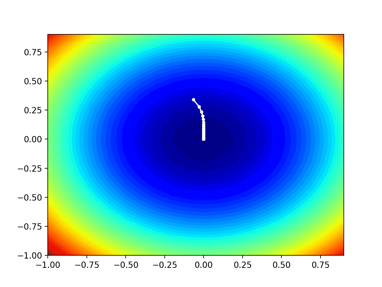
pyplot.show()Running this example performs the search as before, but in this case, a contour map of the objective function is created.
In this case, we can see that each solution found in the search process shows a white point, starting above the optimal value and gradually approaching the optimal value in the center of the graph.