© By Alex

01 introduction

The basic framework of SLAM can be roughly divided into two categories: probability based methods such as EKF, UKF, particle filters and graph based methods. Graph based method is essentially an optimization method, which aims to minimize the observation error of the environment. It is still the core of the mainstream framework. karto, cartographer, hector, etc. are based on optimization. This framework has emerged 20 years ago, such as the famous Atlas, which is still the mainstream today.

The original intention of Atlas is to design a general framework in which to experiment with various mapping algorithms. The purpose is to build small local maps, and then put these small maps together into a large map. To use "nonsense" is to establish a globally consistent map based on the local mapping algorithm under small-scale region and finite calculation.

The name of atlas comes from ancient Greek mythology. The well-known God King Zeus is only the third generation. The first generation is his grandfather Uranus. Zeus and his father Cronus have successively staged dog blood dramas in which his son destroyed Lao Tzu and usurped power. In the Zeus era, the seating on Olympus was basically scheduled. After his father Cronus killed his grandfather Uranus and won the victory, Titan, the leader of the giant family, stood in the wrong team due to mixing with his grandfather, and the loser was Kou. When he settled accounts in autumn, he and his minions were all driven into hell - the dark abyss tartalos. One of the giants, Atlas, was probably picked out to the West because of his size and strength. He stood on Gaia and held Uranus, the heavenly father. The heavenly father was the sky. He could not come down and make trouble there (equivalent to imprisonment). In short, Atlas is the giant standing on the earth to hold the sky, just like Pangu in ancient Chinese mythology.

Well, let's talk about the SLAM framework of Atlas. The idea of the framework is generally to represent the local coordinate system as nodes on the graph. This local coordinate system can be some landmarks, and the transformation between adjacent coordinate systems is represented as edges. The goal is to make all the edges add up to the shortest.

This paper introduces the simplest version of graph based SLAM framework. However, although sparrows are small, they have all kinds of internal organs. After understanding, you can build your own SLAM system on this basis.

02 let's look at the demonstration results first

Blue line: ground truth Intend to go out of such a track

Black line: dead reckoning

Dead reckoning is a method to calculate the position of the next time by measuring the moving distance and orientation under the condition of knowing the position of the current time.

Red line: motion trajectory estimated by algorithm

Anyway, everyone has to go their own way. They can only learn for so limited time. After learning, it's hard to say what the result is. Red is the best result.

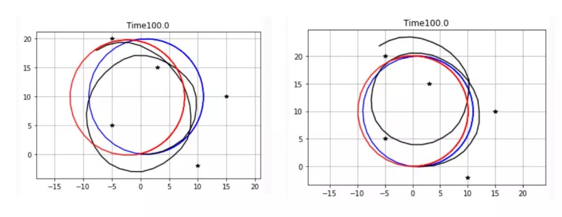
The results of running the same program twice are different, because random noise is added every time, which will lead to different estimation results, as well as in practical application.

03 flow chart and code Notes

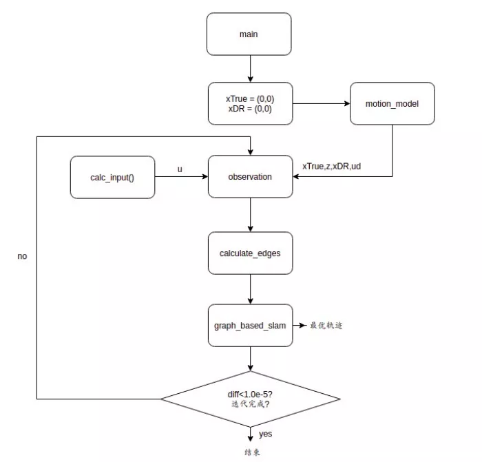
1. Program entry: main() function:

• given road markings: 5 stars

• view these five points in a small car. xTrue: the ground truth starts from (0,0) and the real track xDR starts from (0,0).

· function u = calc_input() calculates the required control vector: velocity = 1m/s, angular velocity = 0.1 rad/s.

· and make an observation xTrue, z, xDR, ud = observation(xTrue, xDR, u, RFID)

• co simulation SIM_TIME = 100 seconds, observe the environment once every DT = 2 seconds, and operate the trolley once.

· first, the control vector needs to be calculated once.

· every show_ graph_ d_ Time = call x once every 20 seconds_ opt = graph_ based_ Slam (hxdr, Hz), 5 times in total, the best path inferred from the current position and historical trajectory, as shown by the red line in the figure.

def main():......# RFID positions [x, y, yaw]Road marking coordinates#The road signs are fixed here#Generally, road signs need to meet four conditions:# 1.Easily repeated observation# 2.There are obvious differences between different road markings# 3.There should be a sufficient number of road markings in the environment# 4.Road sign points should be stable or static, such as eye-catching buildings, traffic signs, etc RFID = np.array([[10.0, -2.0, 0.0],[15.0, 10.0, 0.0],[3.0, 15.0, 0.0],[-5.0, 20.0, 0.0],[-5.0, 5.0, 0.0]])# State Vector [x y yaw v]'xTrue = np.zeros((STATE_SIZE, 1))#ground truthxDR = np.zeros((STATE_SIZE, 1)) # Dead reckoning.That is, the real track of the small car in the program while SIM_TIME >= time:#Simulation 100 seconds...time += DT#Timing, give a control signal to the trolley every two seconds, and observe the environment once d_time += DTu = calc_input()#Generate control signal xTrue, z, xDR, ud = observation(xTrue, xDR, u, RFID)hz.append(z)if d_time >= show_graph_d_time:#Called every 20 seconds graph_based_slam ,Estimate an optimal trajectory x_opt = graph_based_slam(hxDR, hz)#Generate the best trajectory through the real trajectory and the distance to the road sign

2. Observation function

Called every 2 seconds in the main() function, it has two functions:

① Call xTrue = motion_model(xTrue, u) generates ground truth data (no noise in trajectory and control)

② Call xd = motion_model(xd, ud) adds noise to the observation data (both trajectory and control have noise). The next observation will be generated by using the trajectory, real trajectory, control quantity and road signs of the previous time. In practical application, the observation is complex. Observation data are usually derived from various sensors, such as cameras (monocular, binocular), imu, radar, sonar, GPS, etc., and sensors need to be calibrated. Data retrieved from different sensors need simultaneous interpreting. Sensor fusion is also a research hotspot.

def observation(xTrue, xd, u, RFID):xTrue = motion_model(xTrue, u)#Noiseless trajectory and control, call motion model, generate for the next moment groundtruth trajectory# add noise to gps x-yz = np.zeros((0, 4))for i in range(len(RFID[:, 0])):#This cycle is to add noise to the distance and angle between the trolley and the road markings dx = RFID[i, 0] - xTrue[0, 0]#RFID yes main()The coordinates of road markings defined in are fixed dy = RFID[i, 1] - xTrue[1, 0]#xTrue yes ground truth trajectory d = math.hypot(dx, dy)#sqrt(dx^2+dy^2)#Finding distance, Pythagorean theorem angle = pi_2_pi(math.atan2(dy, dx)) - xTrue[2, 0]#Inverse cotangent angle phi = pi_2_pi(math.atan2(dy, dx))#Convert angles to radians if d <= MAX_RANGE:#MAX_RANGE = 30dn = d + np.random.randn() * Q_sim[0, 0] # add noiseangle_noise = np.random.randn() * Q_sim[1, 1]angle += angle_noisephi += angle_noisezi = np.array([dn, angle, phi, i])#Put together an array z = np.vstack((z, zi))# add noise to input Add noise to control signal ud1 = u[0, 0] + np.random.randn() * R_sim[0, 0]ud2 = u[1, 0] + np.random.randn() * R_sim[1, 1]ud = np.array([[ud1, ud2]]).Txd = motion_model(xd, ud)#The real trajectory and noise control signal are used to call the motion model to generate the noisy trajectory at the next time return xTrue, z, xd, ud#

3.motion_model motion model

Aircraft, vehicles and robots have their own motion models, which are used to describe their own unique motion modes, how to convert various control quantities into various motions: how to generate rotor, wheel, displacement or rotation of walking legs, straight travel, turning, overturning and other operations.

4.graph_based_slam(hxDR, hz)

This function is the core of the framework.

The input of the function is historical data, including: ① real trajectory ② output the optimal trajectory from the observation of road signs at each point of the real trajectory.

def graph_based_slam(x_init, hz):print("start graph based slam")z_list = copy.deepcopy(hz)x_opt = copy.deepcopy(x_init)nt = x_opt.shape[1]n = nt * STATE_SIZE for itr in range(MAX_ITR):edges = calc_edges(x_opt, z_list)#Calculate the total cost function H = np.zeros((n, n))b = np.zeros((n, 1))for edge in edges:H, b = fill_H_and_b(H, b, edge)#Extract information matrix# to fix originH[0:STATE_SIZE, 0:STATE_SIZE] += np.identity(STATE_SIZE)dx = - np.linalg.inv(H) @ b#The total cost is associated with the parameters of each point to calculate the amount to be corrected for i in range(nt):x_opt[0:3, i] += dx[i * 3:i * 3 + 3, 0]#Correct the real trajectory and get the optimal trajectory diff = DX T @ dxprint("iteration: %d, diff: %f" % (itr + 1, diff))if diff < 1.0e-5:breakreturn x_ opt

5.calc_edge()

Create graph - graph Each point on the trajectory and each landmark are nodes on the graph. The observation error from the landmark to the trajectory point constitutes an edge cost function.

def calc_edge(x1, y1, yaw1, x2, y2, yaw2, d1,angle1, d2, angle2, t1, t2):edge = Edge()tangle1 = pi_2_pi(yaw1 + angle1)tangle2 = pi_2_pi(yaw2 + angle2)tmp1 = d1 * math.cos(tangle1)tmp2 = d2 * math.cos(tangle2)tmp3 = d1 * math.sin(tangle1)tmp4 = d2 * math.sin(tangle2)edge.e[0, 0] = x2 - x1 - tmp1 + tmp2edge.e[1, 0] = y2 - y1 - tmp3 + tmp4edge.e[2, 0] = 0Rt1 = calc_rotational_matrix(tangle1)Rt2 = calc_rotational_matrix(tangle2)sig1 = cal_observation_sigma()sig2 = cal_observation_sigma()edge.omega = np.linalg.inv(Rt1 @ sig1 @ Rt1.T + Rt2 @ sig2 @ Rt2.T)#Weight matrix edge d1, edge. d2 = d1, d2edge. yaw1, edge. yaw2 = yaw1, yaw2edge. angle1, edge. angle2 = angle1, angle2edge. id1, edge. id2 = t1, t2return edge

6.calc_edges(hxDR, hz)

The contribution of each point on the trajectory to the cost function is calculated, and the total cost function generated by all points on the trajectory is calculated.

def calc_edges(x_list, z_list):edges = [] cost = 0.0z_ids = list(itertools.combinations(range(len(z_list)), 2))for (t1, t2) in z_ids:x1, y1, yaw1 = x_list[0, t1], x_list[1, t1], x_list[2, t1]x2, y2, yaw2 = x_list[0, t2], x_list[1, t2], x_list[2, t2]if z_list[t1] is None or z_list[t2] is None:continue # No observationfor iz1 in range(len(z_list[t1][:, 0])):for iz2 in range(len(z_list[t2][:, 0])):if z_list[t1][iz1, 3] == z_list[t2][iz2, 3]:d1 = z_list[t1][iz1, 0]angle1, phi1 = z_list[t1][iz1, 1], z_list[t1][iz1, 2]d2 = z_list[t2][iz2, 0]angle2, phi2 = z_list[t2][iz2, 1], z_list[t2][iz2, 2]edge = calc_edge(x1, y1, yaw1, x2, y2, yaw2, d1, angle1, d2, angle2, t1, t2)edges.append(edge)cost += (edge.e.T @ edge.omega @ edge.e)[0, 0]print("cost:", cost, ",n_edge:", len(edges))return edges

7. Information matrix and cost function

The information matrix is used to express uncertainty and associate the total cost function with the gradient of each variable:

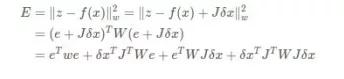
It needs to be completed through the information matrix: the principle of optimal trajectory:

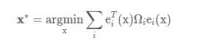
To minimize the total cost function, how to update variables:

The information matrix is the inverse of the covariance matrix.

def fill_H_and_b(H, b, edge):#Calculate the amount of information matrix and update A, B = calc_jacobian(edge)id1 = edge.id1 * STATE_SIZEid2 = edge.id2 * STATE_SIZEH[id1:id1 + STATE_SIZE, id1:id1 + STATE_SIZE] += A.T @ edge.omega @ AH[id1:id1 + STATE_SIZE, id2:id2 + STATE_SIZE] += A.T @ edge.omega @ BH[id2:id2 + STATE_SIZE, id1:id1 + STATE_SIZE] += B.T @ edge.omega @ AH[id2:id2 + STATE_SIZE, id2:id2 + STATE_SIZE] += B.T @ edge.omega @ B b[id1:id1 + STATE_SIZE] += (A.T @ edge.omega @ edge.e)b[id2:id2 + STATE_SIZE] += (B.T @ edge.omega @ edge.e)return H, b stay graph_based_slam()In function: for i in range(nt):x_opt[0:3, i] += dx[i * 3:i * 3 + 3, 0]#Update each point of the actual trajectory to obtain the optimal trajectory

Private letter I receive dry goods learning resources such as target detection and R-CNN / application of data analysis / e-commerce data analysis / application of data analysis in the medical field / NLP student project display / introduction and practical application of Chinese NLP / NLP series live courses / NLP cutting-edge model training camp.