Greenplum real time data warehouse practice -- real time data loading

The previous article explained in detail how to use Canal and Kafka to synchronize MySQL data to Greenplum in real time. According to the first part of this topic Figure 1-1 data warehouse architecture , we have implemented the real-time extraction process of ETL to synchronize data to RDS. This article continues to introduce how to implement the following data loading process. The overall steps to realize real-time data loading can be summarized as follows:

1. Preliminary preparation In order to minimize the stop time of MySQL replication, this step includes all the work that can be completed in the early stage: (1) Create required objects in the target Greenplum, such as dedicated resource queue, schema, transition area table, dimension table and fact table of data warehouse, etc. (2) Preload, such as date dimension data. (3) Configure the table mapping relationship of the Canal Adapter and generate a yml file for each synchronization table.

2. Stop MySQL replication Provides a static data view.

3. Full ETL (1) Perform full synchronization and import the MySQL table data to be synchronized into the transition zone table of Greenplum. (2) Complete the initial load with SQL in Greenplum.

4. Create rule s After full ETL and before real-time ETL, create rule objects in Greenplum to realize automatic real-time loading logic.

5. Restart the Canal Server and the Canal Adapter Prepare to obtain binlog from MySQL database, transfer it through Kafka, and apply the data changes to the transition area table of Greenplum. (1) Stop the Canal Server and delete the meta.dat and h2.mv.db files. If HA is configured, stop all canal servers in the cluster and delete the current synchronization data node in Zookeeper. (2) Stop the Canal Adapter. (3) Start the Canal Server. If HA is configured, start all the canal servers in the cluster. At this time, the incremental data synchronization point will be reset in Zookeeper. (4) Start the Canal Adapter.

6. Start MySQL replication and automatically start real-time ETL. Stop the automatic synchronization of incremental change data during MySQL replication, and trigger the rule to automatically perform real-time loading.

Firstly, we introduce a small and typical sales order example to describe the business scenario, explain the entities and relationships contained in the example, as well as the establishment process of source and target library tables, test data and date dimension generation. Then use Greenplum's SQL script to complete the initial data loading. Finally, the rule object of Greenplum is introduced, and the data is automatically loaded into TDS from RDS in real time by creating rules. Insert a description of the Greenplum technology or object used in creating the example model at any time.

6.1 establish an example data warehouse model

6.1. 1. Business scenario

1. Operational data source

The example operating system is a sales order system. Initially, there are only three tables: product, customer and sales order. The entity relationship diagram is shown in Figure 6-1.

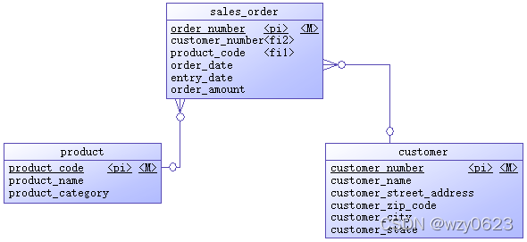
Figure 6-1 data source entity relationship diagram

The tables and their attributes in this scenario are simple. The product table and customer table belong to the basic information table, which store the information of products and customers respectively. Products have only three attributes: product number, product name and product classification. Product number is the primary key and uniquely identifies a product. The customer has six attributes. In addition to the customer number and customer name, it also includes four customer location attributes: Province, city, street and zip code. Customer number is the primary key that uniquely identifies a customer. In practical application, the basic information table is usually maintained by other background systems. The sales order table has six attributes. The order number is the primary key and uniquely identifies a sales order record. Product number and customer number are two foreign keys, which refer to the primary keys of product table and customer table respectively. The other three attributes are order time, registration time and order amount. Order time refers to the time when the customer places an order. Order amount attribute refers to the amount that the order needs to spend. The meaning of these attributes is very clear. Order registration time indicates the time of order entry. In most cases, it should be equal to the order time. If an order needs to be re entered due to a certain situation, the time of the original order and the time of re entry must be recorded at the same time, or some problems occur, and the order registration time lags behind the time of placing the order (this situation will be discussed in the "late facts" section of the fact table technology later in this topic), the two attribute values will be different.

The source system adopts relational model design. In order to reduce the number of tables, this system only achieves 2NF. Region information depends on zip code, so there is transmission dependency in this model.

2. Sales order data warehouse model design

We use 2.2. 1dimensional data model modeling process This paper introduces the four step modeling method to design the star data warehouse model. (1) Select a business process. In this example, only one sales order business process is involved. (2) Declaration granularity. ETL processes in real time and stores the most fine-grained order transaction records in the fact table. (3) Confirmation dimension. Obviously, products and customers are the dimensions of sales orders. The date dimension is used for business integration and provides an important historical perspective for data warehouses. Each data warehouse should have a date dimension. The order dimension is specially designed to describe the degradation dimension technology later. We will introduce the degradation dimension in detail in the dimension table technology of this topic. (4) Confirm the fact. The sales order is the only fact in the current scenario.

The entity relationship diagram of the example data warehouse is shown in Figure 6-2.

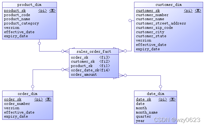
Figure 6-2 entity relationship diagram of data warehouse

As a demonstration example, the entity attributes in the above entity relationship diagram are very simple. You can know their meaning by looking at the attribute name. In addition to the date dimension, the other three dimensions add four attributes: proxy key, version number, effective date and expiration date on the basis of the source data to describe the history of dimension change. When the dimension attribute changes, a new dimension record is generated or the original record is modified according to different strategies. The date dimension has its particularity. Once the dimension data is generated, it will not change, so the version number, effective date and expiration date are not required. The proxy key is the primary key of the dimension table. The fact table refers to the proxy key of the dimension table as its own foreign key. The four foreign keys constitute the joint primary key of the fact table. The order amount is the only measure in the current fact table.

6.1. 2. Establish database table

In order to create a new environment from scratch and avoid data synchronization errors during the establishment of the sample model of real-time data warehouse, stop the running Canal Server (both HA) and Canal Adapter before establishing the library table.

# Both 126 and 127 constituting Canal HA are executed
~/canal_113/deployer/bin/stop.sh
# Query Zookeeper for confirmation
/opt/cloudera/parcels/CDH-6.3.1-1.cdh6.3.1.p0.1470567/lib/zookeeper/bin/zkCli.sh
[zk: localhost:2181(CONNECTED) 0] ls /otter/canal/destinations/example/cluster
[]
# Stop the Canal Adapter and execute
~/canal_113/adapter/bin/stop.sh

1. Create source database objects in MySQL main database and generate test data

(1) Execute the following SQL statement to establish the source database table.

-- Establish the source database and execute it on the main database
drop database if exists source;  
create database source;  
 
use source;  
 
-- Create customer table    
create table customer (    
    customer_number int not null auto_increment primary key comment 'Customer number, primary key',    
    customer_name varchar(50) comment 'Customer name',    
    customer_street_address varchar(50) comment 'Customer address',    
    customer_zip_code int comment 'Zip code',    
    customer_city varchar(30) comment 'City',    
    customer_state varchar(2) comment 'Province'    
);  
 
-- Create product table    
create table product (       
    product_code int not null auto_increment primary key comment 'Product code, primary key',    
    product_name varchar(30) comment 'Product name',    
    product_category varchar(30) comment 'product type'       
);  
 
-- Create sales order table    
create table sales_order (    
    order_number bigint not null auto_increment primary key comment 'Order number, primary key',    
    customer_number int comment 'Customer number',    
    product_code int comment 'Product code',    
    order_date datetime comment 'Order time',    
    entry_date datetime comment 'Registration time',    
    order_amount decimal(10 , 2 ) comment 'sales amount',    
    foreign key (customer_number)    
        references customer (customer_number)    
        on delete cascade on update cascade,    
    foreign key (product_code)    
        references product (product_code)    
        on delete cascade on update cascade    
);

(2) Execute the following SQL statement to generate source library test data

use source;  
 
-- Generate customer table test data    
insert into customer 
(customer_name,customer_street_address,customer_zip_code,
customer_city,customer_state) 
values      
('really large customers', '7500 louise dr.',17050, 'mechanicsburg','pa'),    
('small stores', '2500 woodland st.',17055, 'pittsburgh','pa'),    
('medium retailers','1111 ritter rd.',17055,'pittsburgh','pa'),    
('good companies','9500 scott st.',17050,'mechanicsburg','pa'),    
('wonderful shops','3333 rossmoyne rd.',17050,'mechanicsburg','pa'),    
('loyal clients','7070 ritter rd.',17055,'pittsburgh','pa'),    
('distinguished partners','9999 scott st.',17050,'mechanicsburg','pa');  
 
-- Generate product table test data    
insert into product (product_name,product_category)    
values     
('hard disk drive', 'storage'),    
('floppy drive', 'storage'),    
('lcd panel', 'monitor');  
  
-- Generate 100 sales order table test data  
drop procedure if exists generate_sales_order_data;  
delimiter //    
create procedure generate_sales_order_data()  
begin   
    drop table if exists temp_sales_order_data;  
    create table temp_sales_order_data as select * from sales_order where 1=0;  
  
    set @start_date := unix_timestamp('2021-06-01');  
    set @end_date := unix_timestamp('2021-10-01');  
    set @i := 1;  
  
    while @i<=100 do  
        set @customer_number := floor(1 + rand() * 6);  
        set @product_code := floor(1 + rand() * 2);  
        set @order_date := from_unixtime(@start_date + rand() * (@end_date - @start_date));  
        set @amount := floor(1000 + rand() * 9000);  
  
        insert into temp_sales_order_data values (@i,@customer_number,@product_code,@order_date,@order_date,@amount);  
        set @i:=@i+1;  
    end while;  
  
    truncate table sales_order;  
    insert into sales_order   
    select null,customer_number,product_code,order_date,entry_date,order_amount from temp_sales_order_data order by order_date;  
    commit;  
  
end   
//    
delimiter ;   
  
call generate_sales_order_data();

The test data of customer table and product table are taken from the book Dimensional Data Warehousing with MySQL. We create a MySQL stored procedure to generate 100 sales order test data. In order to simulate the actual order, the customer number, product number, order time and order amount in the order table take random values within a range, and the order time is the same as the registration time. Because the primary key of the order table is self incremented, in order to keep the primary key value consistent with the value order of the order time field, a key named temp is introduced_ sales_ order_ Data table to store intermediate temporary data. Later, this scheme is used to generate order test data.

2. Create the target library object in Greenplum

(1) Create resource queue

# Connect to Greenplum with gpadmin user
psql
-- Create resource queue
create resource queue rsq_dwtest with 
(active_statements=20,memory_limit='8000MB',priority=high,cost_overcommit=true,min_cost=0,max_cost=-1);
-- modify dwtest Resource queue used by users
alter role dwtest resource queue rsq_dwtest;
-- View user resource queue
select rolname, rsqname from pg_roles, pg_resqueue  
 where pg_roles.rolresqueue=pg_resqueue.oid;

Resource group and resource queue are two objects used by Greenplum to manage resources. Resource queue is used by default. All users must be assigned to the resource queue. If they are not specified when creating a user, the user will be assigned to the default resource queue pg_default.

It is recommended to create separate resource queues for different types of workloads. For example, you can create different resource queues for advanced users, WEB users, report management, etc. The appropriate resource queue limit can be set according to the load pressure of the related work.

active_statements controls the maximum number of active statements, which is set to 20, meaning that it is allocated to RSQ_ For all users of dwtest resource queue, at most 20 statements can be executed at the same time. Statements that exceed will be in a wait state until the previous statement being executed has completed.

memory_limit controls the total amount of memory that can be used by the queue. Total memory of all resource queues_ Limit is recommended to be set to less than 90% of the total physical memory available to a Primary node. In this environment, a single machine has 128GB of memory and is configured with 6 Primary nodes. Each Primary node can obtain 21GB of physical memory. If there are multiple resource queues, their memory_ The total limit should not exceed 21GB * 0.9 = 19GB.

When with active_ When statements are used in combination, the default memory allocated for each statement is: memory_limit / active_statements. If a Primary node exceeds the memory limit, the related statements will be canceled, resulting in failure. Therefore, how to configure memory parameters more reasonably and adjust them based on the statistical results of the real production environment is the most stable.

Priority controls the CPU usage priority. The default value is medium. When competing for CPU concurrently, statements in the high priority resource queue will get more CPU resources. For the priority setting of the resource queue to be enforced in the execution statement, you must ensure that GP_ resqueue_ The priority parameter has been set to on.

min_cost and max_cost respectively limits the minimum and maximum costs that can be consumed by the executed statement. Cost is the total estimated cost evaluated by the query optimizer, which means the number of operations on the disk, expressed as a floating-point number. For example, 1.0 is equivalent to obtaining a disk page. In this example, rsq_dwtest is set to unlimited execution cost.

If a resource queue is configured with a Cost threshold, you can set the allowed cost_overcommit. When no other statements are executed in the system, statements exceeding the resource queue Cost threshold can be executed. When there are other statements executing, the Cost threshold is still forcibly evaluated and limited. If Cost_ If overcommit is set to FALSE, statements that exceed the Cost threshold will always be rejected.

(2) Establishing schema in dw Library

# Connect Greenplum with dwtest user
psql -U dwtest -h mdw -d dw
-- establish rds pattern
create schema rds;
-- establish tds pattern
create schema tds;
-- View mode
\dn
-- Modify the schema lookup path of the database
alter database dw set search_path to rds, tds, public, pg_catalog, tpcc_test; 
-- Reconnect dw database
\c dw
-- Display mode find path
show search_path;

Each Greenplum session can only connect to one database at any one time. During ETL processing, rds needs to be associated with the table in tds for query, so it is obviously inappropriate to store rds and tds objects in a separate database. Here, two rds and tds patterns are created in dw database. rds stores the original data as the transition from source data to data warehouse, and tds stores the transformed multidimensional data warehouse. Creating a table in the corresponding mode can make the logical organization of data clearer.

(3) Creating database objects in rds schema

-- Set mode lookup path
set search_path to rds;
 
-- Establish customer original data sheet
create table customer 
( 
  customer_number int primary key,  
  customer_name varchar(30),  
  customer_street_address varchar(30),  
  customer_zip_code int,  
  customer_city varchar(30),  
  customer_state varchar(2)
); 
 
comment on table customer is 'Customer original data sheet';
comment on column customer.customer_number is 'Customer number';
comment on column customer.customer_name is 'Customer name';
comment on column customer.customer_street_address is 'Customer address';
comment on column customer.customer_zip_code is 'Customer zip code';
comment on column customer.customer_city is 'Customer's City';
comment on column customer.customer_state is 'Customer's Province';
 
-- Establish original product data sheet
create table product 
( 
  product_code int primary key, 
  product_name varchar(30),  
  product_category varchar(30)
); 
 
comment on table product is 'Original product data sheet';
comment on column product.product_code is 'Product code';
comment on column product.product_name is 'Product name';
comment on column product.product_category is 'product type';
 
-- Create sales order original data table
create table sales_order
( 
  order_number bigint,    
  customer_number int,    
  product_code int,    
  order_date timestamp,    
  entry_date timestamp,    
  order_amount decimal(10 , 2 ),
  primary key (order_number, entry_date)
) distributed by (order_number)
partition by range (entry_date)  
( start (date '2021-06-01') inclusive    
   end (date '2022-04-01') exclusive    
   every (interval '1 month') ); 
 
comment on table sales_order is 'Sales order original data sheet';
comment on column sales_order.order_number is 'order number';
comment on column sales_order.customer_number is 'Customer number';
comment on column sales_order.product_code is 'Product code';
comment on column sales_order.order_date is 'Order time';
comment on column sales_order.entry_date is 'Registration time';
comment on column sales_order.order_amount is 'sales amount';

The table data in rds mode comes from MySQL tables and is loaded as is without any conversion. Therefore, its table structure is consistent with that in MySQL. The table storage adopts the default row heap mode. For the selection of Greenplum table storage mode, see 3.3. 1 storage mode . When a primary key is defined for a table and no distribution key is specified, Greenplum uses the primary key as the distribution key, which is used for the customer and product tables. As far as Greenplum is concerned, the most important factor to obtain performance is to achieve uniform data distribution. Therefore, the selection of distribution key is very important. It directly affects the data skew, then the processing skew, and finally the query execution speed. Selecting the distribution key should take the calculation of large tasks as the highest goal. The following is the best practice of distribution strategy given by Greenplum.

For any table, specify the distribution key explicitly or use random distribution instead of relying on the default behavior.
If possible, only a single column should be used as the distribution key. If a single column cannot achieve uniform distribution, use the distribution key of up to two columns. More distribution columns usually do not produce a more uniform distribution, and additional time is required in the hashing process.
If the two column distribution key cannot achieve uniform distribution of data, use random distribution. In most cases, multi column distribution keys require a motion operation to join tables, so they have no advantage over random distribution.
The distribution key column data should contain a unique value or a very high cardinality (the ratio of the number of different values to the total number of rows).
If it is not designed for a specific purpose, try not to use the columns that frequently appear in the where query criteria as the distribution key.
You should try to avoid using the date or time column as the distribution key, because this column is generally not used to associate queries with other table columns.
Do not use partition fields as distribution keys.
In order to improve the association performance of large tables, the association columns between large tables should be considered as distribution keys, and the association columns must also be of the same data type. If the associated column data is not distributed in the same segment, the rows required by one table should be dynamically redistributed to other segments. When the connected rows are on the same segment, most of the processing can be done in the segment instance. These connections are called local connections. Local connections minimize data movement. Each network segment operates independently of other network segments. There is no network traffic or communication between network segments.
Regularly check the skew of data distribution and processing. The Greenplum O & M and monitoring section later in this topic will provide more information about checking data skew and processing skew.

rds stores copies of original business data, sales_ The order table contains all orders with a large amount of data. To facilitate the maintenance of large tables, sales_order adopts the design of range partition table. The data is partitioned once a month, and the registration time is used as the partition key. Although sales_order. order_ The value of the number column itself is unique, but similar to the partition table of MySQL, the partition table of Greenplum also requires that the partition key column be included in the primary key, otherwise an error will be reported:

ERROR:  PRIMARY KEY constraint must contain all columns in the partition key
HINT:  Include column "entry_date" in the PRIMARY KEY constraint or create a part-wise UNIQUE index after creating the table instead.

This limitation is related to the implementation of partitioned tables. For the partition table in Greenplum, each partition is physically the same as an ordinary table. The \ d command of psql will list all partition sub table names, and you can directly access these partition sub tables. The partition definition is stored in the system data dictionary table, which logically organizes the partitions together to form a partition table to provide transparent access to the outside world. Unlike Oracle, MySQL and Greenplum partition tables do not have the concept of a global index, and a unique index can only ensure the uniqueness of each partition. Determined by the definition of the partition table, the values of the partition keys are mutually exclusive between partitions. Therefore, adding the partition key column to the primary key can achieve global uniqueness. Moreover, if both a primary key and a distribution key are specified, the distribution key should be a subset of the primary key:

HINT:  When there is both a PRIMARY KEY and a DISTRIBUTED BY clause, the DISTRIBUTED BY clause must be a subset of the PRIMARY KEY.

Because of this implementation of partitioned tables, when multi-level partitions are used, it is easy to produce a large number of partitioned sub tables, which will bring great performance problems and system table pressure. Creating multi-level partitioned tables should be avoided as much as possible.

(4) Creating database objects in tds schema

-- Set mode lookup path
set search_path to tds;
 
-- Create customer dimension table    
create table customer_dim (    
    customer_sk bigserial, 
    customer_number int,    
    customer_name varchar(50),    
    customer_street_address varchar(50),    
    customer_zip_code int,    
    customer_city varchar(30),    
    customer_state varchar(2),  
    version int,  
    effective_dt timestamp,
    expiry_dt timestamp,
    primary key (customer_sk, customer_number)    
) distributed by (customer_number);

-- Create product dimension table    
create table product_dim (    
    product_sk bigserial, 
    product_code int,    
    product_name varchar(30),    
    product_category varchar(30),
    version int,  
    effective_dt timestamp,
    expiry_dt timestamp,
    primary key (product_sk, product_code)    
) distributed by (product_code);  
 
-- Create order dimension table    
create table order_dim (    
    order_sk bigserial,    
    order_number bigint, 
    version int,  
    effective_dt timestamp,
    expiry_dt timestamp,
    primary key (order_sk, order_number)
) distributed by (order_number);
 
-- Create date dimension table  
create table date_dim (      
    date_sk serial primary key,    
    date date,    
    month smallint,    
    month_name varchar(9),    
    quarter smallint,    
    year smallint );   
  
-- Create sales order fact table    
create table sales_order_fact (    
    order_sk bigint,    
    customer_sk bigint,    
    product_sk bigint, 
    order_date_sk int,    
    year_month int,    
    order_amount decimal(10 , 2 ),
    primary key (order_sk, customer_sk, product_sk, order_date_sk, year_month)
) distributed by (order_sk)
partition by range (year_month)  
( partition p202106 start (202106) inclusive ,
  partition p202107 start (202107) inclusive ,
  partition p202108 start (202108) inclusive ,
  partition p202109 start (202109) inclusive ,
  partition p202110 start (202110) inclusive ,
  partition p202111 start (202111) inclusive ,
  partition p202112 start (202112) inclusive ,  
  partition p202201 start (202201) inclusive ,  
  partition p202202 start (202202) inclusive ,  
  partition p202203 start (202203) inclusive   
                     end (202204) exclusive );

Like rds, tables in tds use the default heap storage mode by row. An additional date dimension table is created in tds. The data warehouse can track historical data, so each data warehouse should have a dimension table related to date and time. In order to capture and represent data changes, except for the date dimension table, other dimension tables have four fields more than the source table: proxy key, version number, version effective time and version expiration time. The date dimension will not change after generating data at one time. Therefore, in addition to the related attributes of the date itself, only one column of proxy keys is added. The fact table consists of the proxy key and measurement attribute of the dimension table. Initially, there is only one measurement value of the sales order amount. Users can declare foreign keys and save this information in system tables, but Greenplum does not enforce foreign key constraints.

Due to the large amount of data in the fact table, the range partition table design is adopted. The fact table has a redundant month and year column as the partition key. The reason why the year / month is used as the range partition is that the year / month grouping is often used for query and statistics in data analysis, so that the partition can be effectively used to eliminate and improve the query performance. With RDS sales_ Unlike order, the partition is explicitly defined here.

Load customer_dim,product_dim,order_ When the data of the three dim dimension tables are, it is obviously necessary to associate the primary keys of the corresponding tables in rds, namely customer_number,product_code and order_number. According to the best practice of distribution key, select a single column and use the associated column between tables as the distribution key. Fact table sales_ order_ The data loading of fact needs to be associated with multiple dimension tables, including order_dim is the largest dimension table. Following best practices, we should have chosen order for local correlation_ Number column as sales_ order_ The distribution key of fact, but there is no order in the table_ Number column, which is through order_sk and order_dim dimension table Association. Select order here_ Although SK as a distribution key is unreasonable, it is intentional. When we explain the degradation dimension later in this topic, we will correct this problem.

6.1. 3. Generate date dimension data

Date dimension is a special role in data warehouse. The date dimension contains the concept of time, and time is the most important. Because one of the main functions of data warehouse is to store and trace historical data, the data in each data warehouse has a time characteristic. In this example, a Greenplum function is created to preload the date data at one time.

-- Function to generate date dimension table data  
create or replace function fn_populate_date (start_dt date, end_dt date)    
returns void as $$    
declare    
    v_date date:= start_dt;   
    v_datediff int:= end_dt - start_dt;  
begin    
    for i in 0 .. v_datediff loop      
        insert into date_dim(date, month, month_name, quarter, year)    
        values(v_date, extract(month from v_date), to_char(v_date,'mon'), extract(quarter from v_date), extract(year from v_date));   
        v_date := v_date + 1;  
    end loop;  
    analyze date_dim;  
end; $$    
language plpgsql;

-- Execute function to generate date dimension data
select fn_populate_date(date '2020-01-01', date '2022-12-31');  

-- Query generated date
select min(date_sk) min_sk, min(date) min_date, max(date_sk) max_sk, max(date) max_date, count(*) c 
  from date_dim;

6.2 initial loading

Before the data warehouse can be used, historical data needs to be loaded. These historical data are the first data set imported into the data warehouse. The first load is called the initial load and is generally a one-time job. It is up to the end user to decide how much historical data enters the data warehouse. For example, if the data warehouse starts on December 1, 2021 and the user wants to load historical data for two years, the source data between December 1, 2019 and November 30, 2021 should be loaded initially. All dimension tables must be loaded before loading the fact table. Because the fact table needs to reference the proxy key of the dimension. This is not only for initial loads, but also for periodic loads. This section describes the steps to perform the initial load, including identifying source data, processing dimension history, developing and verifying the initial load process.

6.2. 1 data source mapping

Before the initial loading step of design and development, it is necessary to identify the available source data used by each fact table and each dimension table of the data warehouse, and understand the characteristics of the data source, such as file type, record structure and accessibility. Table 6-1 shows the key information of the source data required by the sales order sample data warehouse, including the source data table, the corresponding data warehouse target table and other attributes. This kind of table is usually called data source correspondence diagram because it reflects the correspondence between each source data and target data. The process of generating this table is called logical data mapping. In this example, the source data of customers and products are directly related to the target table in the data warehouse, customer_dim and product_ The dim table corresponds to the sales order transaction table, which is the data source of multiple data warehouse tables.

Source data	Source data type	File name / table name	Target table in data warehouse
customer	MySQL table	customer	customer_dim
product	MySQL table	product	product_dim
Sales order	MySQL table	sales_order	order_dim,sales_order_fact

Table 6-1 sales order data source mapping

6.2. 2 determine SCD treatment method

The data source is identified. Now consider the processing of dimension history. Most dimension values change over time, such as customer name change, product name or category change, etc. When a dimension changes, for example, when a product has a new classification, it is necessary to record the historical change information of the dimension. In this case, product_ The dim table must store both the old product classification and the current product classification. In addition, the products in the old sales order refer to the old classification. Slow Changing Dimensions (SCD) is a technology to realize dimension history in multidimensional data warehouse. There are three different SCD technologies: SCD type 1 (SCD1), SCD type 2 (SCD2), and SCD type 3 (SCD3):

SCD1 - directly overwrite existing values by updating dimension records. It does not maintain the history of records. SCD1 is generally used to modify incorrect data.
SCD2 - when the source data changes, create a new "version" record for the dimension record to maintain the dimension history. SCD2 does not delete or modify existing data. The table that uses SCD2 to process data change history is sometimes vividly called "zipper table". As the name suggests, the so-called zipper is to record all change information of a piece of data from generation to the current state, and connect the whole life cycle of each record in series like a zipper.
SCD3 – several versions commonly used to maintain dimension records. It maintains history by adding multiple columns to a data unit. For example, in order to record the change of customer address, customer_ The dim dimension table has a customer_ The address column and a previous_ customer_ The address column records the addresses of the current version and the previous version respectively. SCD3 can effectively maintain limited history, rather than saving all history like SCD2. SCD3 is rarely used. It is only applicable when the storage space of data is insufficient and the user accepts the history of limited dimensions.

Different fields in the same dimension table can have different change processing methods. In this example, the customer name of customer dimension history uses SCD1, the customer address uses SCD2, and the two attributes of product dimension, product name and product type use SCD2 to save historical change data. In SQL implementation, SCD1 generally updates attributes directly, while SCD2 adds records.

6.2. 3. Implement proxy key

Dimension tables and fact tables in multidimensional data warehouse generally need a proxy key as the primary key of these tables. The proxy key is generally composed of a single column self increasing number sequence. The bigserial (or serial) data type in Greenplum is similar to auto_increment in MySQL in function and is often used to define self incrementing columns. However, its implementation method is similar to sequence in Oracle. When creating a table with bigserial field, Greenplum will automatically create a self incrementing sequence object, and the bigserial field will automatically reference sequence to realize self incrementing.

The sequence in Greenplum database is essentially a special single line record table, which is used to generate self increasing numbers and self increasing identifiers for the records of the table. Greenplum provides commands to create, modify, and delete sequences. It also provides two built-in functions: nextval() to get the next value of the sequence; setval() resets the initial value of the sequence.

The currval() and lastval() functions of PostgreSQL are not supported in Greenplum, but can be obtained by directly querying the sequence table. For example:

dw=> select last_value, start_value from date_dim_date_sk_seq;
 last_value | start_value 
------------+-------------
       1096 |           1
(1 row)

The sequence object includes several attributes, such as name, step size (amount increased each time), minimum value, maximum value, cache size, etc. there is also a Boolean attribute is_called, which means whether nextval() returns the value first or the value of the sequence increases first. For example, if the current value of the sequence is 100_ If called is TRUE, the next call to nextval() returns 101. If is_ If called is FALSE, the next call to nextval() returns 100.

6.2. 4 perform the initial load

The initial data loading requires two main operations: one is to load the data of MySQL table into the table in RDS mode, and the other is to load the data into the table in TDS mode.

1. Load RDS mode table

It is implemented using the full data synchronization method introduced in the previous article.

-- 127 Stop copying from library
stop slave;
# Export data from library
cd ~
mkdir -p source_bak
mysqldump -u root -p123456 -S /data/mysql.sock -t -T ~/source_bak source customer product sales_order --fields-terminated-by='|' --single-transaction
# Copy the exported data file to the master host of Greenplum
scp ~/source_bak/*.txt gpadmin@114.112.77.198:/data/source_bak/

# Connect to database with gpadmin user
psql -d dw

-- Set search path to rds
set search_path to rds;

-- Empty the table before loading to realize idempotent operation
truncate table customer;    
truncate table product;    
truncate table sales_order;    

-- Load external data into the original data table
copy rds.customer from '/data/source_bak/customer.txt' with delimiter '|';
copy rds.product from '/data/source_bak/product.txt' with delimiter '|';
copy rds.sales_order from '/data/source_bak/sales_order.txt' with delimiter '|';

-- After loading the data, analyze the table before executing the query to improve the query performance
analyze rds.customer;  
analyze rds.product;  
analyze rds.sales_order;

2. Table of loading TDS mode

Connect the Greenplum database with dwtest user and execute the following SQL implementation.

# dwtest user execution
psql -U dwtest -h mdw -d dw

-- Set search path
set search_path to tds, rds;

-- Empty the table before loading to realize idempotent operation
truncate table customer_dim;    
truncate table product_dim;    
truncate table order_dim;    

-- Sequence initialization
alter sequence customer_dim_customer_sk_seq restart with 1;
alter sequence product_dim_product_sk_seq restart with 1;
alter sequence order_dim_order_sk_seq restart with 1;

-- load customer_dim Dimension table
insert into customer_dim (customer_number,customer_name,customer_street_address,customer_zip_code,customer_city,customer_state,version,effective_dt,expiry_dt) 
select customer_number,customer_name,customer_street_address,customer_zip_code,customer_city,customer_state,1,'2021-06-01','2200-01-01'
  from customer;

-- load product_dim Dimension table
insert into product_dim (product_code,product_name,product_category,version,effective_dt,expiry_dt) 
select product_code,product_name,product_category,1,'2021-06-01','2200-01-01'
  from product;

-- load order_dim Dimension table
insert into order_dim (order_number,version,effective_dt,expiry_dt)
select order_number,1,'2021-06-01','2200-01-01'
  from sales_order;

-- load sales_order_fact Fact table
insert into sales_order_fact(order_sk,customer_sk,product_sk,order_date_sk,year_month,order_amount) 
select order_sk, customer_sk, product_sk, date_sk, to_char(order_date, 'YYYYMM')::int, order_amount
  from rds.sales_order a, order_dim b, customer_dim c, product_dim d, date_dim e
 where a.order_number = b.order_number
   and a.customer_number = c.customer_number
   and a.product_code = d.product_code
   and date(a.order_date) = e.date;

-- analysis tds Schema table  
analyze customer_dim;  
analyze product_dim;  
analyze order_dim;  
analyze sales_order_fact;

The purpose of emptying the table before loading and reinitializing the sequence is to repeat the initial loading SQL script. Because the data has been pre generated, the initial loading SQL does not need to process date_dim dimension table. The initial version number of other dimension table data is 1, and the effective time and expiration time are set to the same value, The effective time is earlier than the earliest order generation time (the minimum sales_order.order_date value), and the expiration time is set to a large enough date value. Load all dimension tables first, and then load the fact table. It is a good habit to load a large amount of data and then perform the analysis table operation. It is also a recommended practice of Greenplum, which helps the query optimizer to formulate the best execution plan and improve query performance.

3. Validation data

After the initial load is completed, you can use the following query to verify the correctness of the data.

select order_number,customer_name,product_name,date,
order_amount amount  
  from sales_order_fact a, customer_dim b, product_dim c, 
order_dim d, date_dim e  
 where a.customer_sk = b.customer_sk  
   and a.product_sk = c.product_sk  
   and a.order_sk = d.order_sk  
   and a.order_date_sk = e.date_sk  
 order by order_number;

Note that the proxy key implemented by sequence in this example is different from the business primary key, even if select is used during insertion Order by doesn't help either:

dw=> select order_sk, order_number from order_dim order by order_number limit 5;
 order_sk | order_number 
----------+--------------
       64 |            1
       91 |            2
       90 |            3
       89 |            4
       83 |            5
(5 rows)

Single line insert can ensure sequential increment, for example, 6.1 FN in subsection 3_ populate_ Insert statement used in the date function. Only when a single insert statement inserts multiple records (such as the insert... Select statement used here). This is not a big problem for the data warehouse. Think about the UUID primary key! Let's just remember that the Greenplum sequence only guarantees uniqueness, not sequencing. Therefore, the application logic should not rely on the order of proxy keys. If it is necessary to keep the initially loaded proxy keys in the same order as the business primary key, just write a function or function Name block, use the cursor to traverse the source table records according to the business primary key order, and insert the target table one by one in the loop. For example:

do $$declare
  r_mycur record;   
begin
  --When reading in the cursor, it is best to sort the values first to ensure the order of circular calls
  for r_mycur in select order_number from sales_order order by order_number
  loop 
      --Loop insert within cursor
      insert into order_dim (order_number,version,effective_dt,expiry_dt) 
      values (r_mycur.order_number,1,'2021-06-01','2200-01-01');
  end loop;
end$$;

There are gains and losses. The disadvantage of this scheme is poor performance. At the end of the last article, we tested that Greenplum can execute about 1500 single line DML S per second in this environment, which is much slower than batch processing.

6.3 real time loading

The initial loading is only performed once before the data warehouse is used, while the real-time loading is generally incremental, and the change history of data needs to be captured and recorded. This section describes the steps to perform real-time loading, including identifying source data and loading type, configuring incremental data synchronization, creating Greenplum rule s, and starting and testing the real-time loading process.

6.3. 1. Identify data source and loading type

For real-time loading, first identify the available source data used by each fact table and each dimension table in the data warehouse, and then determine the extraction mode and dimension history loading type suitable for loading. Table 6-2 summarizes this information for this example.

data source	RDS mode	TDS mode	Extraction mode	Dimension history load type
customer	customer	customer_dim	Real time increment	SCD2 on the address column and SCD1 on the name column
product	product	product_dim	Real time increment	All attributes are SCD2
sales_order	sales_order	order_dim	Real time increment	Unique order number
sales_order	sales_order	sales_order_fact	Real time increment	N/A
N/A	N/A	date_dim	N/A	Preload

Table 6-2 real time loading type of sales order

When capturing data changes, you need to compare the current version data of the dimension table with the latest extracted data from the business database. The implementation is to create a rule object in Greenplum to automatically handle data changes. This design can preserve the history of all data changes, because the logic is defined inside the rule and triggered automatically.

The fact table needs to reference the proxy key of the dimension table, and it does not necessarily reference the proxy key of the current version. For example, for some late facts, you must find the dimension version when the fact occurs. Therefore, all version intervals of a dimension should form a continuous and mutually exclusive time range, and each fact data can correspond to the unique version of the dimension. The implementation method is to use the two columns of version effective time and version expiration time in the dimension table. The validity period of any version is a "closed on the left and open on the right" interval, that is, the version includes the effective time but does not include the expiration time. Because ETL granularity is real-time, all data changes will be recorded.

6.3. 2. Configure incremental data synchronization

This step is to synchronize MySQL data to rds schema tables in real time. We have configured Kafka, Canal Server and Canal Adapter as described in the previous article. Now we only need to add the table mapping configuration of the Canal Adapter and generate a yml file for each synchronization table. This example initially needs to be in / home/mysql/canal_113/adapter/conf/rdb directory to create configuration files for three tables:

customer.yml
product.yml
sales_order.yml

customer. The contents of the YML file are as follows:

dataSourceKey: defaultDS
destination: example
groupId: g1
outerAdapterKey: Greenplum
concurrent: true
dbMapping:
  database: source
  table: customer
  targetTable: rds.customer
  targetPk:
    customer_number: customer_number
#  mapAll: true
  targetColumns:
    customer_number: customer_number
    customer_name: customer_name
    customer_street_address: customer_street_address
    customer_zip_code: customer_zip_code
    customer_city: customer_city
    customer_state: customer_state
  commitBatch: 30000 # Size of batch submission

The other two table mapping profiles are similar. The meanings and functions of various configuration items have been described in detail in the previous chapter and will not be repeated.

6.3. 3 create a rule in Greenplum

1. About rule

Canal can obtain, parse and replay MySQL binlog in real time. The whole process is automatically executed and completely transparent to users. To realize the real-time loading of data, it also needs a program that can capture data changes in real time and automatically trigger the execution of ETL logic. In the database, the first thing that can do this is to think of triggers. Unfortunately, Greenplum castrated the trigger at design time, which should be for performance reasons, Because the trigger's row level trigger algorithm (for each row) is absolutely disastrous for massive data. Fortunately, the rule object inherited by Greenplum from PostgreSQL can provide functions similar to triggers at the cost of executing additional statements (for each statement) has better performance and controllability. Basically, rules can be used instead of triggers.

The Greenplum database rules system allows you to define the actions triggered when inserting, updating, or deleting database tables. When a given command is executed on a given table, the rule causes additional or replacement commands to be run. Rules can also be used to implement SQL views, but automatically updated views often outperform explicit rules. It is important to recognize that rules are essentially command conversion mechanisms or command macros, rather than operating independently on each physical line like triggers. The addition or replacement occurs before the execution of the original command.

The syntax for creating a rule is as follows:

CREATE [OR REPLACE] RULE name AS ON event
  TO table_name [WHERE condition] 
  DO [ALSO | INSTEAD] { NOTHING | command | (command; command 
  ...) }

Parameter Description:

Name: the name of the rule to be created. The name of the rule on the same table must be unique. Multiple rules on the same table and the same event type are applied in alphabetical order.
Event: trigger event, which can be one of select, insert, update and delete.
table_name: the name of the table or view to which the rule is applied.
Condition: any SQL condition expression that returns a Boolean value. The conditional expression can only refer to new or old, cannot refer to any other table, and cannot contain aggregate functions. New and old refer to table_ The new and old values of the name table. The new in the insert and update rules is valid to refer to the new row being inserted or updated. Old is valid in update and delete rules to refer to existing rows being updated or deleted.
Instead: indicates to replace the original command with another command instead of executing it. Instead, the original command does not run at all.
Also: indicates that some commands should be run in addition to the original command. If neither also nor instead is specified, the default value is also.
command: one or more commands that make up the behavior of a rule. Valid commands are select, insert, update or delete. You can use the keyword new or old to refer to the values in the table.

The on select rule must be an unconditional instead rule and must have an operation consisting of a single select command. It is not difficult to see that the on select rule can effectively convert a table into a view. The visible content of the view is the row returned by the select command of the rule, not any content stored in the table. Using the create view command to create views is considered better than the on select rule for creating tables.

You can use \ d < table in psql_ Name > view the rules on the specified table, but there is no command to view the rules separately. From this point of view, Greenplum regards rules as attributes on a table rather than a separate object.

2. Create real-time loading rules

(1) customer table delete rule When deleting a piece of data in the customer table, you need to delete the customer_ Customer in dim dimension table_ The expiration time of the current version line corresponding to number is updated to the current time.

create rule r_delete_customer as on delete to customer do also 
(update customer_dim set expiry_dt=now() where customer_number=old.customer_number and expiry_dt='2200-01-01';);

(2) customer table insertion rule When inserting a new piece of data into the customer table, you need to_ A corresponding data is also inserted into the dim dimension table.

create rule r_insert_customer as on insert to customer do also 
(insert into customer_dim (customer_number,customer_name,customer_street_address,customer_zip_code,customer_city,customer_state,version,effective_dt,expiry_dt) 
 values (new.customer_number,new.customer_name,new.customer_street_address,new.customer_zip_code,new.customer_city,new.customer_state,1,now(),'2200-01-01'););

(3) customer table update rule When updating the data in the customer table, you need to perform different operations according to different SCD types. As can be seen from table 6-2, customer_ Customer of dim dimension table_ street_ SCD2, customer is used on the address column_ Use SCD1 on the name column. Therefore, when updating address, you need to expire the current version of the corresponding row, and then insert a new version. When updating name, update customer directly_ Customer of all versions in the row corresponding to the dim dimension table_ Name value.

create rule r_update_customer as on update to customer do also 
(update customer_dim set expiry_dt=now() 
  where customer_number=new.customer_number and expiry_dt='2200-01-01' 
    and customer_street_address <> new.customer_street_address;

insert into customer_dim (customer_number,customer_name,customer_street_address,customer_zip_code,customer_city,customer_state,version,effective_dt,expiry_dt) 
select new.customer_number,new.customer_name,new.customer_street_address,new.customer_zip_code,new.customer_city,new.customer_state,version + 1,expiry_dt,'2200-01-01'
  from customer_dim 
 where customer_number=new.customer_number 
   and customer_street_address <> new.customer_street_address 
   and version=(select max(version) 
                  from customer_dim 
                 where customer_number=new.customer_number);

update customer_dim set customer_name=new.customer_name 
 where customer_number=new.customer_number and customer_name<>new.customer_name);

According to the definition of the rule, if the customer is updated simultaneously in an update customer statement_ street_ Address and customer_name column, in customer_ SCD1 and SCD2 operations will be triggered on the dim dimension table. Do you want to process SCD2 or SCD1 first? To answer this question, let's look at a simple example. Suppose a dimension table contains four fields c1, c2, c3 and c4. c1 is the proxy key, c2 is the business primary key, c3 uses SCD1 and c4 uses SCD2. The source data changes from 1, 2 and 3 to 1, 3 and 4. If SCD1 is processed first and then SCD2 is processed, the data change process of the dimension table is to change from 1, 1, 2 and 3 to 1, 1, 3 and 3, and then add a record 2, 1, 3 and 4. At this time, the two records in the table are 1, 1, 3, 3 and 2, 1, 3 and 4. If SCD2 is processed first and then SCD1 is processed, the data change process is to first add a record 2, 1, 2 and 4, and then change the records 1, 1, 2, 3 and 2, 1, 2 and 4 to 1, 1, 3, 3 and 2, 1, 3 and 4. It can be seen that no matter who comes first, the final result is the same, and there will be a record that has never existed: 1, 1, 3, 3. Because SCD1 does not save historical changes, from the perspective of c2 field alone, the record values of any version are correct without difference. For the c3 field, the value of each version is different, and the records of all versions need to be tracked. From this simple example, we can draw the following conclusion: the processing order of SCD1 and SCD2 is different, but the final result is the same, and both will produce temporary records that do not actually exist. Therefore, functionally, the processing order of SCD1 and SCD2 is not critical. Just remember that for the field of SCD1, the value of any version is correct, and the field of SCD2 needs to track all versions. In terms of performance, it should be better to process SCD1 first because there are fewer updated data rows. In this example, we first deal with SCD2.

(4) product table deletion rule When you delete a piece of data in the product table, you need to delete product_ Product in dim dimension table_ The expiration time of the current version line corresponding to code is updated to the current time.

create rule r_delete_product as on delete to product do also 
(update product_dim set expiry_dt=now() where product_code=old.product_code and expiry_dt='2200-01-01';);

(5) product table insertion rules When you insert a new piece of data into the product table, you need to add data to the product table_ A corresponding data is also inserted into the dim dimension table.

create rule r_insert_product as on insert to product do also 
(insert into product_dim (product_code,product_name,product_category,version,effective_dt,expiry_dt) 
 values (new.product_code,new.product_name,new.product_category,1,now(),'2200-01-01'););

(6) product table update rules As can be seen from table 6-2, product_ SCD2 is used on all non key columns (except product_code) of the dim dimension table.

create rule r_update_product as on update to product do also 
(update product_dim set expiry_dt=now() 
  where product_code=new.product_code 
    and expiry_dt='2200-01-01' 
    and (product_name <> new.product_name or product_category <> new.product_category);

insert into product_dim (product_code,product_name,product_category,version,effective_dt,expiry_dt) 
select new.product_code,new.product_name,new.product_category,version + 1,expiry_dt,'2200-01-01'
  from product_dim 
 where product_code=new.product_code 
   and (product_name <> new.product_name or product_category <> new.product_category)
   and version=(select max(version) 
                  from product_dim 
                 where product_code=new.product_code));

(7) sales_order table insertion rule The loading of the order dimension table is relatively simple because it does not involve the historical change of the dimension. Just insert the new order number into the order_dim table and sales_ order_ Just use the fact table. Note the execution order in the rule. Insert the dimension table first and then the fact table, because the fact table refers to the proxy key of the dimension table.

create rule r_insert_sales_order as on insert to sales_order do also 
(insert into order_dim (order_sk, order_number,version,effective_dt,expiry_dt) 
 values (new.order_number, new.order_number,1,'2021-06-01','2200-01-01');
 
 insert into sales_order_fact(order_sk,customer_sk,product_sk,order_date_sk,year_month,order_amount) 
 select e.order_sk, customer_sk, product_sk, date_sk, to_char(order_date, 'YYYYMM')::int, order_amount
   from rds.sales_order a, customer_dim b, product_dim c, date_dim d, order_dim e
  where a.order_number = new.order_number and e.order_number = new.order_number
    and a.customer_number = b.customer_number and b.expiry_dt = '2200-01-01'
    and a.product_code = c.product_code and c.expiry_dt = '2200-01-01'
    and date(a.order_date) = d.date
 );

6.3. 4 start real-time loading

1. Rebuild topic (optional) If the topic used by Canal has been created in kafka and there is no consumption backlog, this step can be ignored. To avoid confusion with previous messages, it is recommended to re create topic.

export PATH=$PATH:/opt/cloudera/parcels/CDH-6.3.1-1.cdh6.3.1.p0.1470567/lib/kafka/bin/;
kafka-topics.sh --delete --topic example --bootstrap-server 172.16.1.124:9092
kafka-topics.sh --create --topic example --bootstrap-server 172.16.1.124:9092 --partitions 3 --replication-factor 3

2. Start the Canal Server We have configured the Canal Server HA, and the data synchronization sites are recorded in Zookeeper. Delete the current data synchronization point before starting the Canal Server. After the Canal Server is started, the data synchronization start point will be reset to the binlog position when MySQL stops replication from the database.

# Delete the current data synchronization point in Zookeeper
/opt/cloudera/parcels/CDH-6.3.1-1.cdh6.3.1.p0.1470567/lib/zookeeper/bin/zkCli.sh
[zk: localhost:2181(CONNECTED) 0] delete /otter/canal/destinations/example/1001/cursor

# Start the Canal Server and execute it in sequence on 126 and 127 constituting the Canal HA
~/canal_113/deployer/bin/startup.sh

# Query Zookeeper to confirm the starting synchronization site
/opt/cloudera/parcels/CDH-6.3.1-1.cdh6.3.1.p0.1470567/lib/zookeeper/bin/zkCli.sh
[zk: localhost:2181(CONNECTED) 0] get /otter/canal/destinations/example/1001/cursor
{"@type":"com.alibaba.otter.canal.protocol.position.LogPosition","identity":{"slaveId":-1,"sourceAddress":{"address":"node3","port":3306}},"postion":{"gtid":"","included":false,"journalName":"mysql-bin.000001","position":72569,"serverId":126,"timestamp":1640579962000}}

3. Start the Canal Adapter

# Executed at 126
~/canal_113/adapter/bin/startup.sh

4. Start MySQL replication

-- 127 Open replication from library
start slave;

So far, it is ready. Let's conduct some tests to verify whether the real-time data loading is normal.

6.3. 5 test

1. Generate test data

Prepare customer, product and sales order test data in the source database (126) of MySQL.

use source;
  
/*** Changes in customer data are as follows:  
The street number of customer 6 was changed to 7777 ritter rd. (originally 7070 ritter rd), and then change it back to the original value.
Change the name of customer 7 to distinguished agents. (originally distinguished partners)  
Add an eighth customer. 
***/  
update customer set customer_street_address = '7777 ritter rd.' where customer_number = 6 ;  
update customer set customer_street_address = '7070 ritter rd.' where customer_number = 6 ;
update customer set customer_name = 'distinguished agencies' where customer_number = 7 ;  
insert into customer (customer_name, customer_street_address, customer_zip_code, customer_city, customer_state)  
values ('subsidiaries', '10000 wetline blvd.', 17055, 'pittsburgh', 'pa') ;
  
/*** Changes in product data are as follows:  
Change the name of product 3 to flat panel. (originally lcd panel)  
Add a fourth product.  
***/  
update product set product_name = 'flat panel' where product_code = 3 ;  
insert into product (product_name, product_category)  
values ('keyboard', 'peripheral') ;   

/*** Add 16 orders dated December 23, 2021***/
set sql_log_bin = 0;

drop table if exists temp_sales_order_data;
create table temp_sales_order_data as select * from sales_order where 1=0;

set @start_date := unix_timestamp('2021-12-23');
set @end_date := unix_timestamp('2021-12-24');

set @customer_number := floor(1 + rand() * 8);
set @product_code := floor(1 + rand() * 4);
set @order_date := from_unixtime(@start_date + rand() * (@end_date - @start_date));
set @amount := floor(1000 + rand() * 9000);
insert into temp_sales_order_data
values (1,@customer_number,@product_code,@order_date,@order_date,@amount);

... A total of 16 pieces of data are inserted ...

set sql_log_bin = 1;  
insert into sales_order  
select null,customer_number,product_code,order_date,entry_date,order_amount from temp_sales_order_data order by order_date;    
  
commit ;

Recall from the previous article that when we configured the Canal Server, we designated the hash partition as the primary key of the table to ensure the consumption order of the row update corresponding to the same primary key under multiple partitions. Due to temp_ sales_ order_ The data table has no primary key. When the Canal Server writes a message to Kafka, it cannot determine which partition to write to, and a null pointer error will be reported:

2021-12-24 09:23:26.177 [pool-6-thread-1] ERROR com.alibaba.otter.canal.kafka.CanalKafkaProducer - null
java.lang.NullPointerException: null
        at com.alibaba.otter.canal.common.MQMessageUtils.messagePartition(MQMessageUtils.java:441) ~[canal.server-1.1.3.jar:na]
        at com.alibaba.otter.canal.kafka.CanalKafkaProducer.send(CanalKafkaProducer.java:174) ~[canal.server-1.1.3.jar:na]
        at com.alibaba.otter.canal.kafka.CanalKafkaProducer.send(CanalKafkaProducer.java:124) ~[canal.server-1.1.3.jar:na]
        at com.alibaba.otter.canal.server.CanalMQStarter.worker(CanalMQStarter.java:182) [canal.server-1.1.3.jar:na]
        at com.alibaba.otter.canal.server.CanalMQStarter.access$500(CanalMQStarter.java:22) [canal.server-1.1.3.jar:na]
        at com.alibaba.otter.canal.server.CanalMQStarter$CanalMQRunnable.run(CanalMQStarter.java:224) [canal.server-1.1.3.jar:na]
        at java.util.concurrent.ThreadPoolExecutor.runWorker(ThreadPoolExecutor.java:1149) [na:1.8.0_232]
        at java.util.concurrent.ThreadPoolExecutor$Worker.run(ThreadPoolExecutor.java:624) [na:1.8.0_232]
        at java.lang.Thread.run(Thread.java:748) [na:1.8.0_232]

temp_sales_order_data originally serves as a temporary table. Its data changes do not need to be copied to the MySQL slave database, let alone synchronized to the target Greenplum. Therefore, temp is generated_ sales_order_ Close binlog before data in the data table, and send the data to sales_ Open the binlog before inserting data into the order table, which not only solves the problem of error reporting, but also avoids unnecessary binlog and does not affect data synchronization.

2. Confirm that the real-time loading is performed correctly

(1) Query customer dimension table

dw=> select customer_sk, customer_number, customer_name, customer_street_address,version,effective_dt,expiry_dt 
dw->   from customer_dim 
dw->  order by customer_number, version;
 customer_sk | customer_number |     customer_name      | customer_street_address | version |        effective_dt        |         expiry_dt          
-------------+-----------------+------------------------+-------------------------+---------+----------------------------+----------------------------
           3 |               1 | really large customers | 7500 louise dr.         |       1 | 2021-06-01 00:00:00        | 2200-01-01 00:00:00
           7 |               2 | small stores           | 2500 woodland st.       |       1 | 2021-06-01 00:00:00        | 2200-01-01 00:00:00
           6 |               3 | medium retailers       | 1111 ritter rd.         |       1 | 2021-06-01 00:00:00        | 2200-01-01 00:00:00
           1 |               4 | good companies         | 9500 scott st.          |       1 | 2021-06-01 00:00:00        | 2200-01-01 00:00:00
           5 |               5 | wonderful shops        | 3333 rossmoyne rd.      |       1 | 2021-06-01 00:00:00        | 2200-01-01 00:00:00
           2 |               6 | loyal clients          | 7070 ritter rd.         |       1 | 2021-06-01 00:00:00        | 2021-12-22 13:14:54.194449
           9 |               6 | loyal clients          | 7777 ritter rd.         |       2 | 2021-12-22 13:14:54.194449 | 2021-12-22 13:14:54.194449
          10 |               6 | loyal clients          | 7070 ritter rd.         |       3 | 2021-12-22 13:14:54.194449 | 2200-01-01 00:00:00
           4 |               7 | distinguished agencies | 9999 scott st.          |       1 | 2021-06-01 00:00:00        | 2200-01-01 00:00:00
           8 |               8 | subsidiaries           | 10000 wetline blvd.     |       1 | 2021-12-22 13:14:54.086822 | 2200-01-01 00:00:00
(10 rows)

It can be seen that customer 6 has added two versions due to address change. The expiration time of the previous version is the same as the effective time of the next adjacent version. The validity period of any version is a "closed left and open right" range. The name change of customer 7 directly overwrites the original value and adds customer 8. Note that from effective_dt and customer_ As can be seen from SK, the target database contains customer 8 inserted first and customer 6 updated later. When generating test data, we update customer 6 first and then insert customer 8. As in the previous article 5.6 As mentioned in the discussion of the Canal consumption order in Section 2, selecting the primary key hash method can only ensure the order of multiple binlog s of a primary key. For different primary keys, different orders may be executed at both ends of the source and target. Pay special attention when considering business requirements.

(2) Query product dimension table

dw=> select * from product_dim order by product_code, version;
 product_sk | product_code |  product_name   | product_category | version |        effective_dt        |         expiry_dt          
------------+--------------+-----------------+------------------+---------+----------------------------+----------------------------
          1 |            1 | hard disk drive | storage          |       1 | 2021-06-01 00:00:00        | 2200-01-01 00:00:00
          3 |            2 | floppy drive    | storage          |       1 | 2021-06-01 00:00:00        | 2200-01-01 00:00:00
          2 |            3 | lcd panel       | monitor          |       1 | 2021-06-01 00:00:00        | 2021-12-22 13:15:04.050588
          5 |            3 | flat panel      | monitor          |       2 | 2021-12-22 13:15:04.050588 | 2200-01-01 00:00:00
          4 |            4 | keyboard        | peripheral       |       1 | 2021-12-22 13:15:03.977177 | 2200-01-01 00:00:00
(5 rows)

It can be seen that the name of product 3 is changed, a version is added using SCD2, and the record of product 4 is added.

(3) Query order dimension table

dw=> select * from order_dim order by order_number;
 order_sk | order_number | version |    effective_dt     |      expiry_dt      
----------+--------------+---------+---------------------+---------------------
       64 |            1 |       1 | 2021-06-01 00:00:00 | 2200-01-01 00:00:00
       91 |            2 |       1 | 2021-06-01 00:00:00 | 2200-01-01 00:00:00
       90 |            3 |       1 | 2021-06-01 00:00:00 | 2200-01-01 00:00:00
       89 |            4 |       1 | 2021-06-01 00:00:00 | 2200-01-01 00:00:00
       83 |            5 |       1 | 2021-06-01 00:00:00 | 2200-01-01 00:00:00
...
      111 |          111 |       1 | 2021-06-01 00:00:00 | 2200-01-01 00:00:00
      112 |          112 |       1 | 2021-06-01 00:00:00 | 2200-01-01 00:00:00
      113 |          113 |       1 | 2021-06-01 00:00:00 | 2200-01-01 00:00:00
      114 |          114 |       1 | 2021-06-01 00:00:00 | 2200-01-01 00:00:00
      115 |          115 |       1 | 2021-06-01 00:00:00 | 2200-01-01 00:00:00
      116 |          116 |       1 | 2021-06-01 00:00:00 | 2200-01-01 00:00:00
(116 rows)

Now there are 116 orders, 100 are initially loaded and 16 are loaded in real time. During the initial loading, there are multiple inserts, and the proxy keys are out of order. During the real-time loading, there is a single insert, and the proxy keys are in the same order as the order number.

(4) Query fact table

dw=> select a.order_sk, order_number,customer_name,product_name,date,order_amount
dw->   from sales_order_fact a, customer_dim b, product_dim c, order_dim d, date_dim e
dw->  where a.customer_sk = b.customer_sk
dw->    and a.product_sk = c.product_sk
dw->    and a.order_sk = d.order_sk
dw->    and a.order_date_sk = e.date_sk
dw->  order by order_number;
 order_sk | order_number |     customer_name      |  product_name   |    date    | order_amount 
----------+--------------+------------------------+-----------------+------------+--------------
...
      101 |          101 | distinguished agencies | keyboard        | 2021-12-23 |      5814.00
      102 |          102 | subsidiaries           | keyboard        | 2021-12-23 |      4362.00
      103 |          103 | distinguished agencies | hard disk drive | 2021-12-23 |      3214.00
      104 |          104 | subsidiaries           | keyboard        | 2021-12-23 |      6034.00
      105 |          105 | wonderful shops        | floppy drive    | 2021-12-23 |      8323.00
      106 |          106 | subsidiaries           | keyboard        | 2021-12-23 |      9223.00
      107 |          107 | really large customers | floppy drive    | 2021-12-23 |      5435.00
      108 |          108 | loyal clients          | floppy drive    | 2021-12-23 |      3094.00
      109 |          109 | really large customers | hard disk drive | 2021-12-23 |      8271.00
      110 |          110 | subsidiaries           | hard disk drive | 2021-12-23 |      3463.00
      111 |          111 | loyal clients          | keyboard        | 2021-12-23 |      2022.00
      112 |          112 | medium retailers       | flat panel      | 2021-12-23 |      1125.00
      113 |          113 | good companies         | hard disk drive | 2021-12-23 |      2552.00
      114 |          114 | small stores           | hard disk drive | 2021-12-23 |      5222.00
      115 |          115 | good companies         | hard disk drive | 2021-12-23 |      7801.00
      116 |          116 | really large customers | hard disk drive | 2021-12-23 |      3525.00
(116 rows)

From customer_name,product_name,order_ From the SK field value, you can see that all new orders refer to the latest dimension proxy key.

6.4 dynamic zone scrolling

rds.sales_order and TDS sales_ order_ Facts are partitioned on a monthly basis, and the rolling partition maintenance strategy needs to be further designed. By maintaining a data scrolling window, delete old partitions, add new partitions, and migrate the data of old partitions to secondary storage outside the data warehouse to save system overhead. The following Greenplum function dynamically scrolls partitions according to the steps of dumping the oldest partition data, deleting the oldest partition data and creating a new partition.

-- Function to create dynamic scrolling partitions  
create or replace function tds.fn_rolling_partition(p_year_month_start date) returns int as $body$    
declare    
    v_min_partitiontablename name;  
    v_year_month_end date := p_year_month_start + interval '1 month';  
    v_year_month_start_int int := extract(year from p_year_month_start) * 100 + extract(month from p_year_month_start);  
    v_year_month_end_int int := extract(year from v_year_month_end) * 100  + extract(month from v_year_month_end);  
    sqlstring varchar(1000);      
begin   
    -- handle rds.sales_order  
    -- Dump the data of the earliest month,    
    select partitiontablename into v_min_partitiontablename  
      from pg_partitions    
     where tablename='sales_order' and partitionrank = 1;  
   
    sqlstring = 'copy (select * from ' || v_min_partitiontablename || ') to ''/home/gpadmin/sales_order_' || cast(v_year_month_start_int as varchar) || '.txt'' with delimiter ''|'';';    
    execute sqlstring;    
    -- raise notice '%', sqlstring;    
    
    -- Delete the partition corresponding to the earliest month    
    sqlstring := 'alter table sales_order drop partition for (rank(1));';    
    execute sqlstring;    
        
    -- Add new partition for next month    
    sqlstring := 'alter table sales_order add partition start (date '''|| p_year_month_start ||''') inclusive end (date '''||v_year_month_end  ||''') exclusive;';    
    execute sqlstring;    
    -- raise notice '%', sqlstring;      

       
    -- handle tds.sales_order_fact       
    -- Dump the data of the earliest month,    
    select partitiontablename into v_min_partitiontablename  
      from pg_partitions    
     where tablename='sales_order_fact' and partitionrank = 1;  
   
    sqlstring = 'copy (select * from ' || v_min_partitiontablename || ') to ''/home/gpadmin/sales_order_fact_' || cast(v_year_month_start_int as varchar) || '.txt'' with delimiter ''|'';';    
    execute sqlstring;    
    -- raise notice '%', sqlstring;    
    
    -- Delete the partition corresponding to the earliest month    
    sqlstring := 'alter table sales_order_fact drop partition for (rank(1));';    
    execute sqlstring;    
        
    -- Add new partition for next month    
    sqlstring := 'alter table sales_order_fact add partition start ('||cast(v_year_month_start_int as varchar)||') inclusive end ('||cast(v_year_month_end_int as varchar)||') exclusive;';    
    execute sqlstring;    
    -- raise notice '%', sqlstring;   

    -- Normal return 1    
    return 1;    
        
-- Exception returned 0    
exception when others then     
    raise exception '%: %', sqlstate, sqlerrm;      
    return 0;    
end    
$body$ language plpgsql;

Put the psql command line that executes the function into cron for automatic execution. The following example shows that the partition scrolling operation is performed at 2:00 on the 1st of each month. It is assumed that only the sales data of the last year is retained in the data warehouse.

0 2 1 * * psql -d dw -c "set search_path=rds,tds; select fn_rolling_partition(date(date_trunc('month',current_date) + interval '1 month'));" > rolling_partition.log 2>&1

Summary

We use a simple and typical sales order example to establish a data warehouse model.
In this example model, the source database table is established in MySQL, the RDS and TDS modes are established in Greenplum, the synchronization table is stored in RDS, and the data warehouse table is stored in TDS.
The initial loading is relatively simple. As long as there is a static data view on the source side, it can be implemented in traditional SQL.
With Greenplum rule, automatic real-time data loading of multidimensional data warehouse can be realized.
For partition tables, Greenplum recommends creating only one level of partitions, which usually requires periodic dynamic partition rolling maintenance.

Programmer Think